ePSproc LF/AF function verification & tests
- 10/09/20 v5 AF code now working and verified.
- 27/08/20 v4 Revisiting again, updates to normalisation with degen factor. Now getting correct \(\beta\) values, still some possible issues with total XS however.
- 06/07/20 v3 Updated plotting codes & added AF tests.
- 26/06/20 v2
- 19/06/20 v1
For LF and AF calculations, trying to get to the bottom of issues with magnitudes and/or phases and/or formalism differences with raw ePS matrix elements.
Formalism
Test cases:
- ePS matrix elements with formalism from [1], for LF cross-sections and \(\beta_{2}\). Formalism with Clebsch-Gordan (CG) terms.
- ePSproc AF calculations, for LF cross-sections and \(\beta_{2}\) in isotropic case (or other terms in general cases). Usual 3j-symbol based formalism.
The AF calculations should reduce to the LF case for an isotropic ensemble, and both cases should match the “direct” ePS GetCro outputs (LF). Hopefully this should clear up any outstanding issues with normalisation, units, scale-factors, phase conventions etc. For details of the AF code, see the method dev notes.
(For MF verification, see the MFPADs and associated :math:beta_{LM}` <https://epsproc.readthedocs.io/en/dev/demos/ePSproc_BLM_calc_demo_Sept2019.html#Benchmark-vs.->`__ notebooks, where the numerics are verified for the NO2 test case, although the total cross-sections may still have issues (for more discussion, see the Matlab code release software paper). The geometric tensor version of the MF calculations is also verified against the same test case.)
[1] Cross section and asymmetry parameter calculation for sulfur 1s photoionization of SF6, A. P. P. Natalense and R. R. Lucchese, J. Chem. Phys. 111, 5344 (1999), http://dx.doi.org/10.1063/1.479794
[2] Reid, Katharine L., and Jonathan G. Underwood. “Extracting Molecular Axis Alignment from Photoelectron Angular Distributions.” The Journal of Chemical Physics 112, no. 8 (2000): 3643. https://doi.org/10.1063/1.480517.
[3] Underwood, Jonathan G., and Katharine L. Reid. “Time-Resolved Photoelectron Angular Distributions as a Probe of Intramolecular Dynamics: Connecting the Molecular Frame and the Laboratory Frame.” The Journal of Chemical Physics 113, no. 3 (2000): 1067. https://doi.org/10.1063/1.481918.
[4] Stolow, Albert, and Jonathan G. Underwood. “Time-Resolved Photoelectron Spectroscopy of Non-Adiabatic Dynamics in Polyatomic Molecules.” In Advances in Chemical Physics, edited by Stuart A. Rice, 139:497–584. Advances in Chemical Physics. Hoboken, NJ, USA: John Wiley & Sons, Inc., 2008. https://doi.org/10.1002/9780470259498.ch6.
Formalism: LF case with CG terms
As given in ref. [1]. This is now implemented in implemented in ``ePSproc.lfblmGeom` <https://epsproc.readthedocs.io/en/dev/modules/epsproc.geomFunc.lfblmGeom.html>`__. NOTE - that the \(M\) term here is an MF projection term, and should be summed over for the final LF result.
The matrix elements \(I_{\mathbf{k},\hat{n}}^{(L,V)}\) of Eqs. (8) and (9) can be expanded in terms of the \(X_{lh}^{p\mu}\) functions of Eq. (7) as\(^{14}\)
{[}Note here the final term gives polarization (dipole) terms, with \(l=1\), \(h=v\), corresponding to a photon with one unit of angular momentum and projections \(v=-1,0,1\), correlated with irreducible representations \(p_{v}\mu_{v}\).{]}
The differential cross section is given by
where the asymmetry parameter can be written as\(^{14}\)
and the \((l'lm'm|L'M')\) are the usual Clebsch–Gordan coefficients. The total cross section is
where c is the speed of light.
Additional notes:
- In the current numerics, the XS is defined as \(\beta_0\) calculated as per above, for \(L=0\), or as \(1/3*\sum_{p\mu lhv}|I_{\mathbf{k},\hat{n}}^{(L,V)}|^{2}\). These are identical.
- The normalisation factors of 1/3 and 1/5 appear to be \(1/(2L+1)\) (or other degeneracy - possibly symmetry) terms - TBC.
- Computing \(\beta_0\) with the full formalism gives the correct values here, while using the matrix elements directly requires the additional 1/3 normalisation term.
- For \(\beta_2\), the 1/5 term is required in both cases.
AF formalism
The original (full) form for the AF equations, as implemented in ``ePSproc.afblm` <https://epsproc.readthedocs.io/en/dev/modules/epsproc.AFBLM.html>`__ (NOTE - there are some corrections to be made here, which are not yet implemented in the base code, but are now in the geometric version):
Where \(I_{l,m,\mu}^{p_{i}\mu_{i},p_{f}\mu_{f}}(E)\) are the energy-dependent dipole matrix elements, and \(A_{Q,S}^{K}(t)\) define the alignment parameters.
In terms of the geometric parameters, this can be rewritten as:
See the method dev notebook for more details. Both methods gave the same results for N2 test cases, so are at least consistent, but do not currently match ePS GetCro outputs for the LF case.
Numerics
In both LF and AF cases, the numerics tested herein are based on the geometric tensor expansion code, which has been verified for the MF case as noted above (for PADs at a single energy).
A few additional notes on the implementations…
- The matrix elements used are taken from the DumpIdy output segments of the ePS output file, which provide “phase corrected and properly normalized dynamical coefs”.
- The matrix elements output by ePS are assumed to correspond to \(I_{lhv}^{p\mu(L,V)}\) as defined above.
- The Scale Factor (SF) “to sqrt Mbarn” output with the matrix elements is assumed to correspond to the \(\frac{4\pi^{2}}{3c}E\) term defined above, plus any other required numerical factors (\(4\pi\) terms and similar).
- The SF is energy dependent, but not continuum (or partial wave) dependent.
- If correct, then using matrix elements * scale factor, should give correct results (as a function of \(E\)), while omitting the scale factor should still give correct PADs at any given \(E\), but incorrect total cross-section and energy scaling.
- This may be incorrect, and some other assumptions are tested herein.
- EDIT: now verified as \(SF*\sqrt(4*pi)\) to match LF/GetCro cross-section results.
- The AF and LF case should match for an isotropic distribution, defined as \(A^{0}_{0,0}=1\). Additional normalisation required here…?
- A factor of \(\sqrt{(2K+1)}/8\pi^2\) might be required for correct normalisation, although shouldn’t matter in this case. (See eqn. 47 in [4].)
- For the LF case, as defined above, conversion from Legendre-normalised \(\beta\) to spherical harmonic normalised \(\beta\) is required for comparison with the AF formalism, where \(\beta^{Sph}_{L,0} = \sqrt{(2L+1)/4\pi}\beta^{Lg}\)
Status
09/09/20 - AF code now working correctly, and verified herein, ePSproc v1.2.5-dev.
Set up
[1]:
# Imports
import numpy as np
import pandas as pd
import xarray as xr

# Special functions
# from scipy.special import sph_harm
import spherical_functions as sf
import quaternion

# Performance & benchmarking libraries
# from joblib import Memory
# import xyzpy as xyz
import numba as nb

# Timings with ttictoc or time
# https://github.com/hector-sab/ttictoc
# from ttictoc import TicToc
import time

# Package fns.
# For module testing, include path to module here
import sys
import os

if sys.platform == "win32":
    modPath = r'D:\code\github\ePSproc'  # Win test machine
else:
    modPath = r'/home/femtolab/github/ePSproc/'  # Linux test machine

sys.path.append(modPath)
import epsproc as ep
# TODO: tidy this up!
from epsproc.util import matEleSelector
from epsproc.geomFunc import geomCalc, geomUtils
from epsproc.geomFunc.lfblmGeom import lfblmXprod

# Plotters
from epsproc.plot import hvPlotters
* pyevtk not found, VTK export not available.
[2]:
hvPlotters.setPlotters()
# import bokeh
# import holoviews as hv
# hv.extension('bokeh')


[3]:
# With hvplot.
# This is nice for Bokeh back-end, but a bit of a pain for formatting the plot initially.
# Needs unstacked dims, plus array name.

from hvplot import hvPlot
import hvplot.xarray
Test N2 case
Load data
[4]:
# Load data from modPath\data
dataPath = os.path.join(modPath, 'data', 'photoionization')
dataFile = os.path.join(dataPath, 'n2_3sg_0.1-50.1eV_A2.inp.out')  # Set for sample N2 data for testing

# Scan data file
dataSet = ep.readMatEle(fileIn = dataFile)
dataXS = ep.readMatEle(fileIn = dataFile, recordType = 'CrossSection')  # XS info currently not set in NO2 sample file.
*** ePSproc readMatEle(): scanning files for DumpIdy segments.

*** Scanning file(s)
['D:\\code\\github\\ePSproc\\data\\photoionization\\n2_3sg_0.1-50.1eV_A2.inp.out']

*** Reading ePS output file:  D:\code\github\ePSproc\data\photoionization\n2_3sg_0.1-50.1eV_A2.inp.out
Expecting 51 energy points.
Expecting 2 symmetries.
Scanning CrossSection segments.
Expecting 102 DumpIdy segments.
Found 102 dumpIdy segments (sets of matrix elements).

Processing segments to Xarrays...
Processed 102 sets of DumpIdy file segments, (0 blank)
*** ePSproc readMatEle(): scanning files for CrossSection segments.

*** Scanning file(s)
['D:\\code\\github\\ePSproc\\data\\photoionization\\n2_3sg_0.1-50.1eV_A2.inp.out']

*** Reading ePS output file:  D:\code\github\ePSproc\data\photoionization\n2_3sg_0.1-50.1eV_A2.inp.out
Expecting 51 energy points.
Expecting 2 symmetries.
Scanning CrossSection segments.
Expecting 3 CrossSection segments.
Found 3 CrossSection segments (sets of results).
Processed 3 sets of CrossSection file segments, (0 blank)
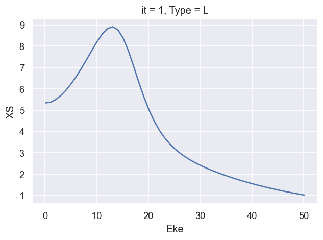
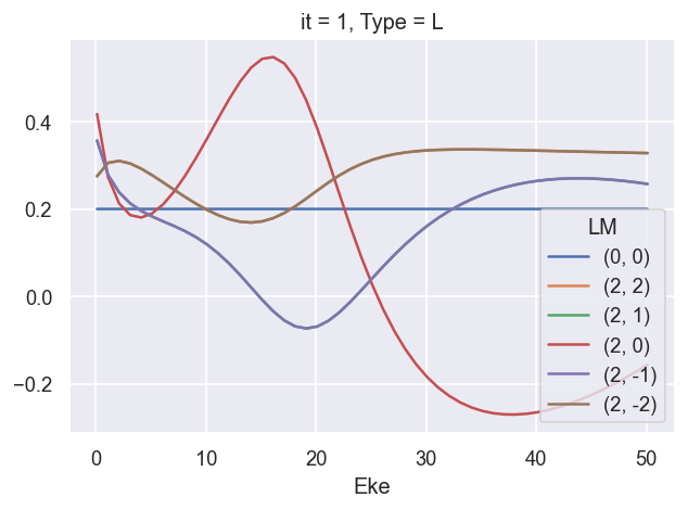
Reference results from GetCro
These are the LF cross-sections and \(\beta\) parameters output directly from ePolyScat, use these as reference results.
[5]:
# Plot cross sections using Xarray functionality
dataXS[0].sel({'Type':'L', 'XC':'SIGMA'}).plot.line(x='Eke');
[6]:
# Plot B2
dataXS[0].sel({'Type':'L', 'XC':'BETA'}).plot.line(x='Eke');
Test LF calculations (CG version)
Without sym summation
[7]:
dataSet[0].coords
[7]:
Coordinates:
    Ehv      (Eke) float64 15.68 16.68 17.68 18.68 ... 62.68 63.68 64.68 65.68
  * LM       (LM) MultiIndex
  - l        (LM) int64 1 1 1 3 3 3 5 5 5 7 7 7 9 9 9 11 11 11
  - m        (LM) int64 -1 0 1 -1 0 1 -1 0 1 -1 0 1 -1 0 1 -1 0 1
  * it       (it) int64 1
  * Type     (Type) object 'L' 'V'
  * mu       (mu) int64 -1 0 1
  * Eke      (Eke) float64 0.1 1.1 2.1 3.1 4.1 5.1 ... 46.1 47.1 48.1 49.1 50.1
  * Sym      (Sym) MultiIndex
  - Cont     (Sym) object 'SU' 'PU'
  - Targ     (Sym) object 'SG' 'SG'
  - Total    (Sym) object 'SU' 'PU'
    SF       (Eke) complex128 (2.1560627+3.741674j) ... (4.4127053+1.8281945j)
[8]:
# Set parameters
SFflag = False  # Multiply matrix elements by SF?
symSum = False  # Sum over symmetries?
phaseConvention = 'S'
thres = 1e-4
selDims = {'it':1, 'Type':'L'}
thresDims = 'Eke'

# Set terms for testing - NOTE ORDERING HERE may affect CG term!!!
dlistMatE = ['lp', 'l', 'L', 'mp', 'm', 'M']  # Match published terms
dlistP = ['p1', 'p2', 'L', 'mup', 'mu', 'M']
# dlistMatE = ['l', 'lp', 'L', 'm', 'mp', 'M']  # Standard terms
# dlistP = ['p1', 'p2', 'L', 'mu', 'mup', 'M']


# Set matrix elements
matE = dataSet[0].copy()

# Calculate betas - dev code has various output types for testing
BetaNormXS, BetaNorm, BetaRaw, XSmatE, BetaNormX = lfblmXprod(matE, symSum = symSum, SFflag = SFflag,
                              thres = thres, thresDims = thresDims, selDims = selDims,
                              phaseConvention = phaseConvention,
                              dlistMatE = dlistMatE, dlistP = dlistP)

# Here BetaNormXS includes the correct normalisation term as per the original formalism, and XSmatE is the sum of the squared matrix elements, as used for the normalisation (== cross section without correct scaling).
# BetaNorm is calculated only from the BLM CG formalism.
[9]:
# Plot results - full XS
plotThres = None
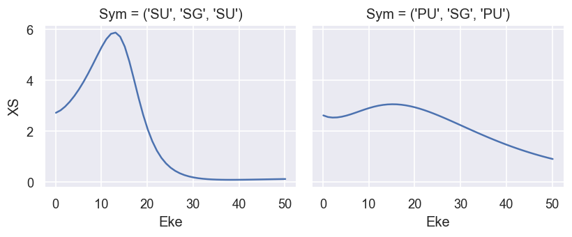
ep.util.matEleSelector(BetaNorm['XS'], thres = plotThres, dims='Eke', sq=True, drop=True).real.plot.line(x='Eke', col='Sym');
[10]:
# Plot results - normalised (B0, B2).
# NOTE - M term here is additional degen factor, as noted above.
# Summing over M gives the final LF terms, as defined above.
# The B0 term (==cross section) is not correctly scaled here.
# The B2 term matches the GetCro reference results.
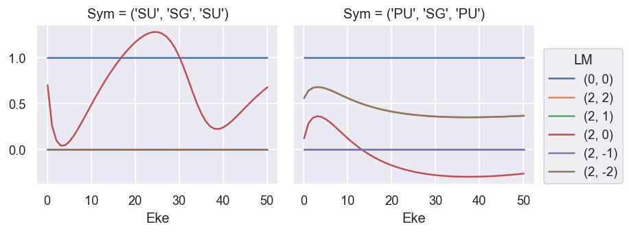
ep.util.matEleSelector(BetaNorm, thres = plotThres, dims='Eke', sq=True, drop=True).real.plot.line(x='Eke', col='Sym'); # Full set of terms
ep.util.matEleSelector(BetaNorm.unstack('LM').sum('M'), thres = plotThres, dims='Eke', sq=True, drop=True).real.plot.line(x='Eke', col='Sym'); # Summed over 'M'
Compare with GetCro reference values
[11]:
# Compare XS values
# Comparison plot using hvplot - needs some work!

xPlot1 = ep.util.matEleSelector(BetaNorm['XS'], thres = plotThres, dims='Eke', sq=True, drop=True).unstack().squeeze() #
xPlot1.name='XS calc'
plot1 = xPlot1.real.unstack().squeeze().hvplot.line(x='Eke', by = 'Total', width=1200, height= 800);  # For hvplot need to unstack & squeeze to avoid dim issues and related errors.
# ep.util.matEleSelector(BetaNormXS_sph, thres = plotThres, dims='Eke', sq=True, drop=True).real.plot.line(x='Eke', linestyle='dashed');

# Ugly sub-select on syms to ensure consistency over data - should be a neater way to do this!
syms = ['SU','PU']
xPlot2 = dataXS[0].sel({'Type':'L', 'XC':'SIGMA'}).unstack().sel({'Total':syms, 'Cont':syms}).squeeze();
# xPlot2 = ep.util.matEleSelector(BetaNormXS_sph, thres = plotThres, dims='Eke', sq=True, drop=True)
xPlot2.name='XS GetCro'
plot2 = xPlot2.real.unstack().squeeze().hvplot.line(x='Eke', by='Total', line_dash='dashed');

(plot1 * plot2)
[11]:
*** OK - the cross-sections from the full CG-calculation and ePS GetCro match for each continuum.
[12]:
# Compare B2 values
# Comparison plot using hvplot - needs some work!

xPlot1 = ep.util.matEleSelector(BetaNorm.unstack('LM').sum('M'), thres = plotThres, dims='Eke', sq=True, drop=True).sel(L=2).unstack().squeeze() #
xPlot1.name='XS calc'
plot1 = xPlot1.real.unstack().squeeze().hvplot.line(x='Eke', by = 'Total', width=1200, height= 800);  # For hvplot need to unstack & squeeze to avoid dim issues and related errors.
# ep.util.matEleSelector(BetaNormXS_sph, thres = plotThres, dims='Eke', sq=True, drop=True).real.plot.line(x='Eke', linestyle='dashed');

# Ugly sub-select on syms to ensure consistency over data - should be a neater way to do this!
syms = ['SU','PU']
xPlot2 = dataXS[0].sel({'Type':'L', 'XC':'BETA'}).unstack().sel({'Total':syms, 'Cont':syms}).squeeze();
# xPlot2 = ep.util.matEleSelector(BetaNormXS_sph, thres = plotThres, dims='Eke', sq=True, drop=True)
xPlot2.name='XS GetCro'
plot2 = xPlot2.real.unstack().squeeze().hvplot.line(x='Eke', by='Total', line_dash='dashed');

(plot1 * plot2)
[12]:
*** OK - the \(\beta_2\) values from the full CG-calculation and ePS GetCro match for each continuum.
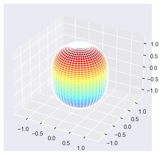
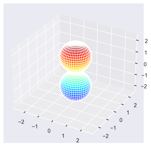
Plot some LFPADs…
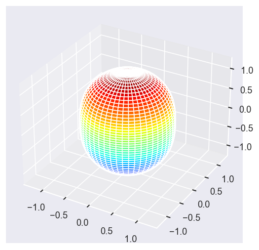
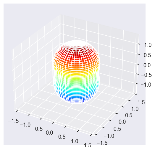
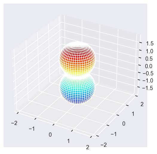
[13]:
Eke = [1.1, 3.1, 25.1, 39.1]
# betaPlot = BetaNormX.sel(Eke=Eke)
betaPlot = BetaNormX.sel(Eke=Eke, Cont='SU', Total='SU').squeeze()

# surfs = ep.sphFromBLMPlot(betaPlot, res = 50, pType = 'r', plotFlag = True, facetDim = 'Eke', backend = 'mpl', fnType = 'lg');
surfs = ep.sphFromBLMPlot(betaPlot, res = 50, pType = 'r', plotFlag = True, facetDim = 'Eke', backend = 'mpl');
Using lg betas (from BLMX array).
Plotting with mpl
Data dims: ('Eke', 'Theta', 'Phi'), subplots on Eke
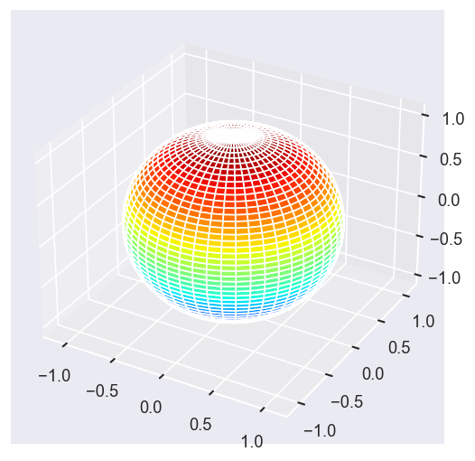
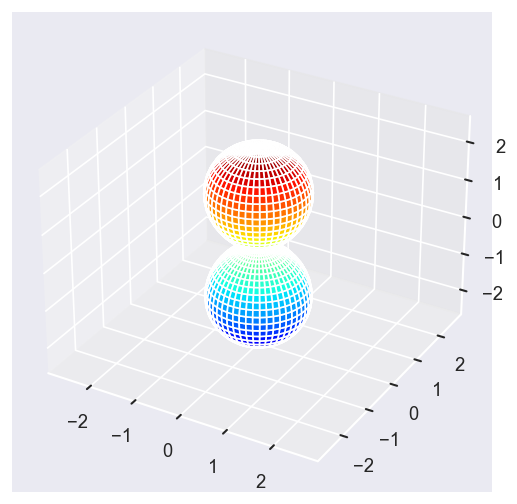
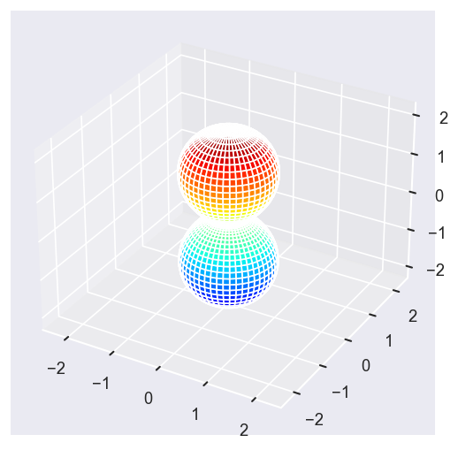
[14]:
# Eke = [1.1, 25.1, 39.1]
# betaPlot = BetaNormX.sel(Eke=Eke)
betaPlot = BetaNormX.sel(Eke=Eke, Cont='PU', Total='PU').squeeze()
surfs = ep.sphFromBLMPlot(betaPlot, res = 50, pType = 'r', plotFlag = True, facetDim = 'Eke', backend = 'mpl', fnType = 'lg');
Using lg betas (as passed).
Plotting with mpl
Data dims: ('Eke', 'Theta', 'Phi'), subplots on Eke
With sym summation
[15]:
# Set parameters
SFflag = False  # Multiply matrix elements by SF?
symSum = True  # Sum over symmetries?
phaseConvention = 'S'
thres = 1e-4
selDims = {'it':1, 'Type':'L'}
thresDims = 'Eke'

# Set terms for testing - NOTE ORDERING HERE may affect CG term!!!
dlistMatE = ['lp', 'l', 'L', 'mp', 'm', 'M']  # Match published terms
dlistP = ['p1', 'p2', 'L', 'mup', 'mu', 'M']
# dlistMatE = ['l', 'lp', 'L', 'm', 'mp', 'M']  # Standard terms
# dlistP = ['p1', 'p2', 'L', 'mu', 'mup', 'M']


# Set matrix elements
matE = dataSet[0].copy()

# Calculate betas
BetaNormXS, BetaNorm, BetaRaw, XSmatE, BetaNormX = lfblmXprod(matE, symSum = symSum, SFflag = SFflag,
                              thres = thres, thresDims = thresDims, selDims = selDims,
                              phaseConvention = phaseConvention,
                              dlistMatE = dlistMatE, dlistP = dlistP)

# Here BetaNormXS includes the correct normalisation term as per the original formalism, and XSmatE is the sum of the squared matrix elements, as used for the normalisation (== cross section without correct scaling).
# BetaNorm is calculated only from the BLM CG formalism.
[16]:
plotThres = None

# ep.util.matEleSelector(XSmatE, thres = plotThres, dims='Eke', sq=True, drop=True).real.plot.line(x='Eke');
ep.util.matEleSelector(BetaNorm['XS'], thres = plotThres, dims='Eke', sq=True, drop=True).real.plot.line(x='Eke');
[17]:
ep.util.matEleSelector(BetaNormXS, thres = plotThres, dims='Eke', sq=True, drop=True).real.plot.line(x='Eke');
[18]:
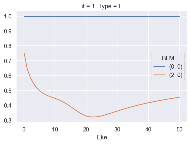
# Summing over M gives the final LF terms, as defined above.
# The B0 term is normalised to unity here.
# The B2 term matches the GetCro reference results.
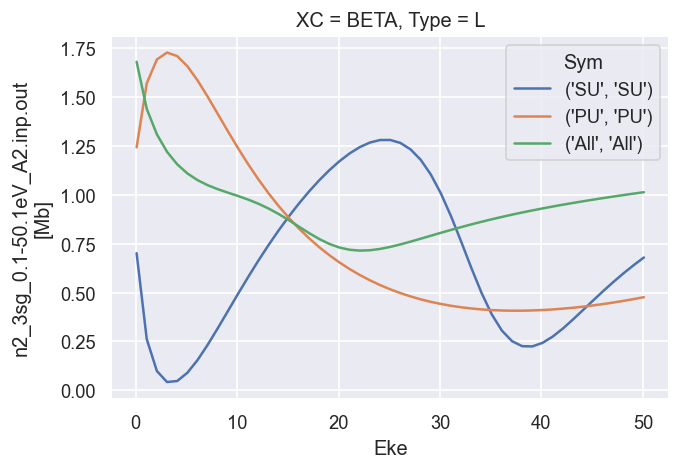
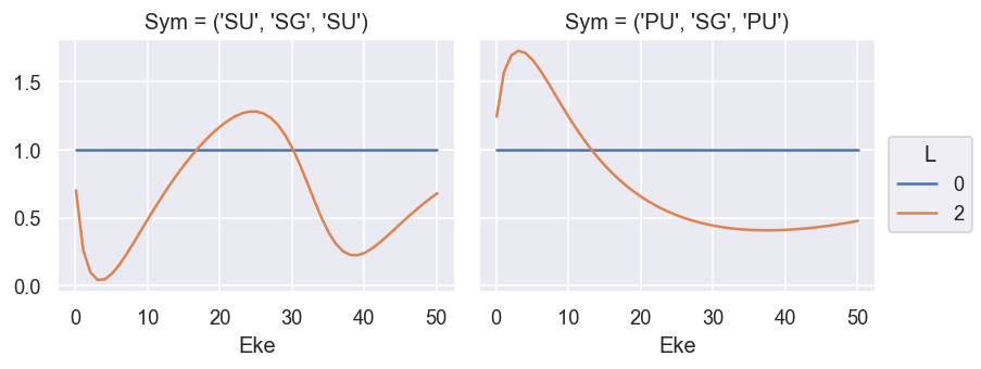
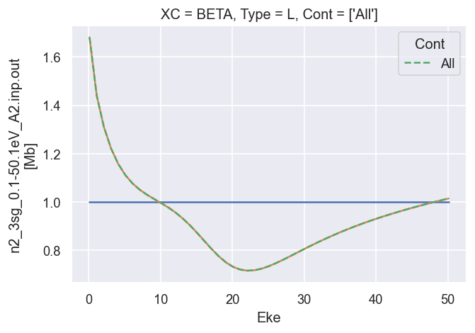
ep.util.matEleSelector(BetaNorm.unstack('LM').sum('M'), thres = plotThres, dims='Eke', sq=True, drop=True).real.plot.line(x='Eke', linestyle = 'solid'); # Now fixed in source
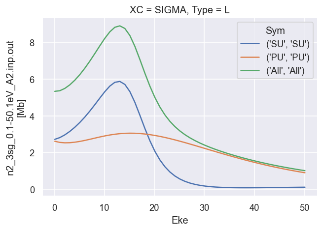
dataXS[0].sel({'Type':'L', 'XC':'BETA', 'Total':'All'}).plot.line(x='Eke', linestyle='dashed'); # Reference results
[19]:
# Check imaginary values... should be ~0
ep.util.matEleSelector(BetaNorm.unstack('LM').sum('M'), thres = plotThres, dims='Eke', sq=True, drop=True).imag.plot.line(x='Eke', linestyle = 'solid');  # Now fixed in source
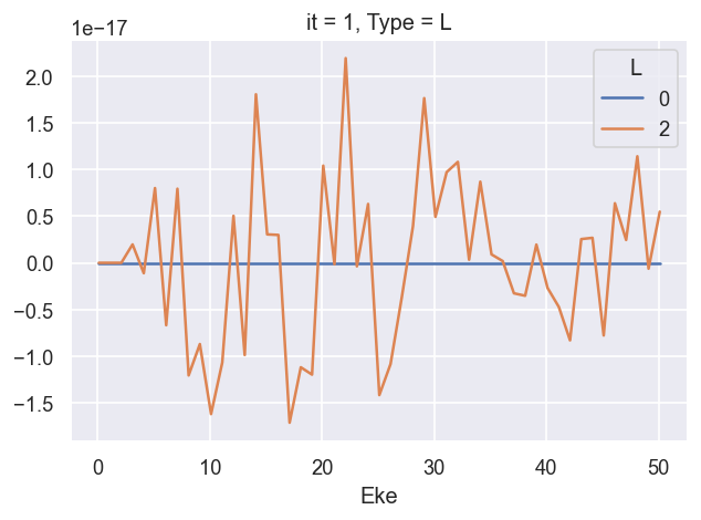
*** 26/06/20 LF CG calcs OK for \(\beta_2\), still need to fix cross-section scaling.
*** 02/09/20 Fixed XS scaling.
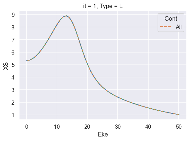
Compare with GetCro reference values
[20]:
# Compare XS values
# Comparison plot using hvplot - needs some work!
plotThres = None
xPlot1 = ep.util.matEleSelector(BetaNorm['XS'], thres = plotThres, dims='Eke', sq=True, drop=True).unstack().squeeze() #
xPlot1.name='XS calc'
plot1 = xPlot1.real.unstack().squeeze().hvplot.line(x='Eke', width=1200, height= 800);  # For hvplot need to unstack & squeeze to avoid dim issues and related errors.
# ep.util.matEleSelector(BetaNormXS_sph, thres = plotThres, dims='Eke', sq=True, drop=True).real.plot.line(x='Eke', linestyle='dashed');

# Ugly sub-select on syms to ensure consistency over data - should be a neater way to do this!
syms = ['All']
xPlot2 = dataXS[0].sel({'Type':'L', 'XC':'SIGMA'}).unstack().sel({'Total':syms, 'Cont':syms}).squeeze();
# xPlot2 = ep.util.matEleSelector(BetaNormXS_sph, thres = plotThres, dims='Eke', sq=True, drop=True)
xPlot2.name='XS GetCro'
plot2 = xPlot2.real.unstack().squeeze().hvplot.line(x='Eke', by='Total', line_dash='dashed');

(plot1 * plot2)
[20]:
*** OK - the cross-sections from the full CG-calculation and ePS GetCro matches.
[21]:
# Compare B2 values
# Comparison plot using hvplot - needs some work!

xPlot1 = ep.util.matEleSelector(BetaNorm.unstack('LM').sum('M'), thres = plotThres, dims='Eke', sq=True, drop=True).sel(L=2).unstack().squeeze() #
xPlot1.name='XS calc'
plot1 = xPlot1.real.unstack().squeeze().hvplot.line(x='Eke', width=1200, height= 800);  # For hvplot need to unstack & squeeze to avoid dim issues and related errors.
# ep.util.matEleSelector(BetaNormXS_sph, thres = plotThres, dims='Eke', sq=True, drop=True).real.plot.line(x='Eke', linestyle='dashed');

# Ugly sub-select on syms to ensure consistency over data - should be a neater way to do this!
syms = ['All']
xPlot2 = dataXS[0].sel({'Type':'L', 'XC':'BETA'}).unstack().sel({'Total':syms, 'Cont':syms}).squeeze();
# xPlot2 = ep.util.matEleSelector(BetaNormXS_sph, thres = plotThres, dims='Eke', sq=True, drop=True)
xPlot2.name='XS GetCro'
plot2 = xPlot2.real.unstack().squeeze().hvplot.line(x='Eke', by='Total', line_dash='dashed');

(plot1 * plot2)
[21]:
*** OK - the \(\beta_2\) from the full CG-calculation and ePS GetCro match for each continuum.
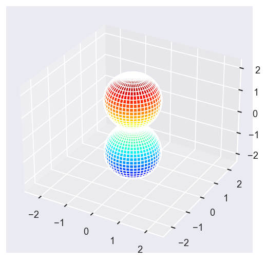
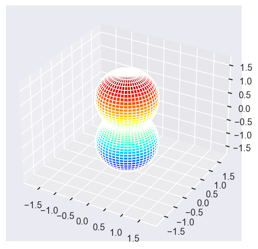
Plot some LFPADs…
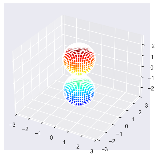
[22]:
Eke = [1.1, 3.1, 25.1, 39.1]
betaPlot = BetaNormX.sel(Eke=Eke)
# betaPlot = BetaNormX.sel(Eke=Eke, Cont='SU', Total='SU').squeeze()
# surfs = ep.sphFromBLMPlot(betaPlot, res = 50, pType = 'r', plotFlag = True, facetDim = 'Eke', backend = 'mpl', fnType = 'lg');
surfs = ep.sphFromBLMPlot(betaPlot, res = 50, pType = 'r', plotFlag = True, facetDim = 'Eke', backend = 'mpl');
Using lg betas (from BLMX array).
Plotting with mpl
Data dims: ('Eke', 'Theta', 'Phi'), subplots on Eke
Conversion & normalisation
This result is \(\beta_2\) for a Legendre Polynomial expansion, as shown above: \(\beta^{Sph}_{L,0} = \sqrt{(2L+1)/4\pi}\beta^{Lg}\). This will allow for comparison with usual AF formalism.
Test:
- Conversion to \(Y_{L,M}\) form.
- LF-PADs to check numerics.
- Confirm total cross-section value & normalisation.
[23]:
# Check value for XS
# BetaNormXS.unstack('LM').sum('M').sel({'L':0})

# FACTOR OF 3 - just degeneracy term in summation.  WHAT ABOUT SF...?
((XSmatE)).real.plot.line(x='Eke')

# Compare with reference results
(dataXS[0].sel({'Type':'L', 'XC':'SIGMA', 'Sym':'All'})).plot.line(x='Eke', linestyle='dashed');

# OK

# Try also vs. vanilla calc...
ep.util.matEleSelector(BetaNorm['XS'], thres = plotThres, dims='Eke', sq=True, drop=True).real.plot.line(x='Eke', linestyle='dotted');
# OK
[24]:
# BetaNorm_sph = ep.conversion.conv_BL_BLM(BetaNorm.unstack('LM').sum('M'), to='sph')
BetaNormX_sph = ep.conversion.conv_BL_BLM(BetaNormX, to='sph', renorm=True)
[25]:
# Check conversion to Sph normalised betas
# ep.util.matEleSelector(BetaNormXS_sph, thres = plotThres, dims='Eke', sq=True, drop=True).real.plot.line(x='Eke');
# ep.util.matEleSelector(BetaNorm_sph, thres = plotThres, dims='Eke', sq=True, drop=True).real.plot.line(x='Eke');
ep.util.matEleSelector(BetaNormX_sph, thres = plotThres, dims='Eke', sq=True, drop=True).real.plot.line(x='Eke');
Q: is \(\beta_{0,0} = \sqrt{1/4\pi}\) value meaningful here, or an issue? Should renorm or otherwise set this to 1? XS should be conserved… is this indicative of another missing/assumed normalisation term? Sph normalisation choice? YES - matches definition for orthonormal sph, see https://docs.scipy.org/doc/scipy/reference/generated/scipy.special.sph_harm.html and https://shtools.github.io/SHTOOLS/complex-spherical-harmonics.html#supported-normalizations.
NOTE - in previous cases this has been normalised away, but significant in cases where XS is preserved.
UPDATE - this is now fixed in ep.conversion.conv_BL_BLM. Default will output values for which full expansions matche (i.e. Pl==Yl expansion), which results in \(\beta^{sph}_{0,0}=\sqrt(4\pi)\) for \(\beta^{lg}_{0}=1\). If renorm=True is set (default case), then values are renormalised to \(\beta_{0}=1\).
Test vs. AF code
Should be identical for unaligned case.
06/07/20 - quick testing, things are CLOSE to reference results above, but there still seems to be inconsistencies somewhere, possibly in renorm only?
01/09/20 - now looking OK for LF (isotropic) case, although renorm per \(L\) may still be off.
09/09/20 - now working correctly, including SF.
[26]:
phaseConvention = 'E'  # Set phase conventions used in the numerics - for ePolyScat matrix elements, set to 'E', to match defns. above.

symSum = True  # Sum over symmetry groups, or keep separate?
SFflag = False  # Include scaling factor to Mb in calculation?

SFflagRenorm = False  # Renorm terms
BLMRenorm = 1

thres = 1e-6
RX = ep.setPolGeoms()  # Set default pol geoms (z,x,y), or will be set by mfblmXprod() defaults - FOR AF case this is only used to set 'z' geom for unity wigner D's - should rationalise this!

selDims = {'it':1, 'Type':'L'}
thresDims = 'Eke'

start = time.time()
mTermST, mTermS, mTermTest, BetaNormX = ep.geomFunc.afblmXprod(dataSet[0], QNs = None, RX=RX, thres = thres, selDims = selDims, thresDims=thresDims,
                                                    symSum=symSum, SFflag=SFflag, phaseConvention=phaseConvention, BLMRenorm=BLMRenorm)
end = time.time()
print('Elapsed time = {0} seconds, for {1} energy points, {2} polarizations, threshold={3}.'.format((end-start), mTermST.Eke.size, RX.size, thres))

# Elapsed time = 3.3885273933410645 seconds, for 51 energy points, 3 polarizations, threshold=0.01.
# Elapsed time = 5.059587478637695 seconds, for 51 energy points, 3 polarizations, threshold=0.0001.
Elapsed time = 3.8381855487823486 seconds, for 51 energy points, 3 polarizations, threshold=1e-06.
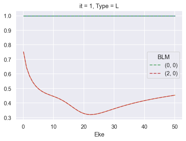
[27]:
# 09/09/20 - updating here for BetaNormX values...

ep.util.matEleSelector(BetaNormX, thres = plotThres, dims='Eke', sq=True, drop=True).real.plot.line(x='Eke');  # Values from AF code
ep.util.matEleSelector(BetaNormX_sph, thres = plotThres, dims='Eke', sq=True, drop=True).real.plot.line(x='Eke', linestyle='dashed');  # Values from LF code.

###### B2 OK!!!!!!!!!!!!!!!!!!!!!!!!!!!!!!!!!!!!!!!!!!!!!!
# BLMRenorm = 1 OK (renorm by XS only, SFflag True or False OK)
# BLMRenorm = 2 FAIL
# BLMRenorm = 3 FAIL (B00 = 2, B20 renorm off by ~2. something)
# BLMRenorm = 4 FAIL (B00 = 2, B20 renorm off by ~2. something)
[28]:
# 09/09/20 - updating here for BetaNormX values...

ep.util.matEleSelector(BetaNormX['XSraw'], thres = plotThres, dims='Eke', sq=True, drop=True).real.plot.line(x='Eke');  # Values from AF code - note these are too small
ep.util.matEleSelector(BetaNormX['XSrescaled'], thres = plotThres, dims='Eke', sq=True, drop=True).real.plot.line(x='Eke');  # Values from AF code *sqrt(4pi) - real valued, match LF code
ep.util.matEleSelector(BetaNormX['XSiso'], thres = plotThres, dims='Eke', sq=True, drop=True).real.plot.line(x='Eke');  # Values from sum over matrix elements - real valued, match LF code

# Ref. values from LF code
ep.util.matEleSelector(BetaNormX_sph['XS'], thres = plotThres, dims='Eke', sq=True, drop=True).real.plot.line(x='Eke', linestyle='dashed');  # Values from LF code.

###### XS OK!!!!!!!!!!!!!!!!!!!!!!!!!!!!!!!!!!!!!!!!!!!!!!
# Now set with:
#  - XSraw = direct AF calculation output.
#  - XSrescaled = XSraw * SF * sqrt(4pi)
#  - XSiso = direct sum over matrix elements
[41]:
# Check imaginary values... should be ~0
ep.util.matEleSelector(BetaNormX, thres = plotThres, dims='Eke', sq=True, drop=True).imag.plot.line(x='Eke', linestyle = 'solid');
# OK
[42]:
# Check imaginary values for XS terms... should be ~0
print(f"Raw imag max: {BetaNormX['XSraw'].imag.max()}")
print(f"Rescaled imag max: {BetaNormX['XSrescaled'].imag.max()}")
print(f"XSiso imag max: {BetaNormX['XSiso'].imag.max()}")

ep.util.matEleSelector(BetaNormX['XSraw'], thres = plotThres, dims='Eke', sq=True, drop=True).imag.plot.line(x='Eke', linestyle = 'solid');
ep.util.matEleSelector(BetaNormX['XSrescaled'], thres = plotThres, dims='Eke', sq=True, drop=True).imag.plot.line(x='Eke', linestyle = 'dashed');
ep.util.matEleSelector(BetaNormX['XSiso'], thres = plotThres, dims='Eke', sq=True, drop=True).imag.plot.line(x='Eke', linestyle = 'dotted');

# OK.
Raw imag max: <xarray.DataArray 'XSraw' ()>
array(0.)
Coordinates:
    Euler    object (0.0, 0.0, 0.0)
    Labels   <U18 'z'
    it       int64 1
    Type     <U1 'L'
Rescaled imag max: <xarray.DataArray 'XSrescaled' ()>
array(0.)
Coordinates:
    Euler    object (0.0, 0.0, 0.0)
    Labels   <U18 'z'
    it       int64 1
    Type     <U1 'L'
XSiso imag max: <xarray.DataArray 'XSiso' ()>
array(0.)
Coordinates:
    Euler    object (0.0, 0.0, 0.0)
    Labels   <U18 'z'
    it       int64 1
    Type     <U1 'L'
Version info
[31]:
import scooby
scooby.Report(additional=['epsproc', 'xarray', 'holoviews'])
[31]:
| Thu Sep 10 18:02:14 2020 Eastern Daylight Time | |||||
| OS | Windows | CPU(s) | 32 | Machine | AMD64 |
| Architecture | 64bit | RAM | 63.9 GB | Environment | Jupyter |
| Python 3.7.3 (default, Apr 24 2019, 15:29:51) [MSC v.1915 64 bit (AMD64)] | |||||
| epsproc | 1.2.5-dev | xarray | 0.15.0 | holoviews | 1.13.3 |
| numpy | 1.19.1 | scipy | 1.3.0 | IPython | 7.12.0 |
| matplotlib | 3.3.1 | scooby | 0.5.6 | ||
| Intel(R) Math Kernel Library Version 2020.0.0 Product Build 20191125 for Intel(R) 64 architecture applications | |||||