Matrix element LM plotting routines demo
28/11/19 v1, 07/02/20 updated Euler grouping,
Source notebook on Github.
Basic IO
[1]:
import sys
import os
import time
import numpy as np

# For module testing, include path to module here
modPath = r'D:\code\github\ePSproc'
# modPath = r'/home/femtolab/github/ePSproc/'
sys.path.append(modPath)
import epsproc as ep
* pyevtk not found, VTK export not available.
[2]:
# Load data from modPath\data
dataPath = os.path.join(modPath, 'data', 'photoionization')
dataFile = os.path.join(dataPath, 'n2_3sg_0.1-50.1eV_A2.inp.out')  # Set for sample N2 data for testing

# Scan data file
dataSet = ep.readMatEle(fileIn = dataFile)
dataXS = ep.readMatEle(fileIn = dataFile, recordType = 'CrossSection')  # XS info currently not set in NO2 sample file.
*** ePSproc readMatEle(): scanning files for DumpIdy segments.

*** Scanning file(s)
['D:\\code\\github\\ePSproc\\data\\photoionization\\n2_3sg_0.1-50.1eV_A2.inp.out']

*** Reading ePS output file:  D:\code\github\ePSproc\data\photoionization\n2_3sg_0.1-50.1eV_A2.inp.out
Expecting 51 energy points.
Expecting 2 symmetries.
Scanning CrossSection segments.
Expecting 102 DumpIdy segments.
Found 102 dumpIdy segments (sets of matrix elements).

Processing segments to Xarrays...
Processed 102 sets of DumpIdy file segments, (0 blank)
*** ePSproc readMatEle(): scanning files for CrossSection segments.

*** Scanning file(s)
['D:\\code\\github\\ePSproc\\data\\photoionization\\n2_3sg_0.1-50.1eV_A2.inp.out']

*** Reading ePS output file:  D:\code\github\ePSproc\data\photoionization\n2_3sg_0.1-50.1eV_A2.inp.out
Expecting 51 energy points.
Expecting 2 symmetries.
Scanning CrossSection segments.
Expecting 3 CrossSection segments.
Found 3 CrossSection segments (sets of results).
Processed 3 sets of CrossSection file segments, (0 blank)
[3]:
jobInfo = ep.headerFileParse(dataFile)
molInfo = ep.molInfoParse(dataFile)
*** Job info from file header.
ePS n2, batch n2_3sg_0.1-50.1eV, orbital A2
N2 X-state (3sg-1)
E=0.1:1.0:50.1 (51 points)
Fri Nov 30 08:47:52 EST 2018
*** Found orbitals
1 1 Ene = -15.6719 Spin =Alpha Occup = 2.000000
2 2 Ene = -15.6676 Spin =Alpha Occup = 2.000000
3 3 Ene = -1.4948 Spin =Alpha Occup = 2.000000
4 4 Ene = -0.7687 Spin =Alpha Occup = 2.000000
5 5 Ene = -0.6373 Spin =Alpha Occup = 2.000000
6 6 Ene = -0.6283 Spin =Alpha Occup = 2.000000
7 7 Ene = -0.6283 Spin =Alpha Occup = 2.000000
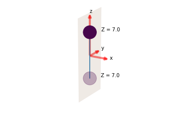
*** Found atoms
Z = 7 ZS = 7 r = 0.0000000000 0.0000000000 0.5328050000
Z = 7 ZS = 7 r = 0.0000000000 0.0000000000 -0.5328050000
[4]:
ep.jobSummary(jobInfo, molInfo);
*** Job summary data
 ePS n2, batch n2_3sg_0.1-50.1eV, orbital A2
 N2 X-state (3sg-1)
 E=0.1:1.0:50.1 (51 points)
 Fri Nov 30 08:47:52 EST 2018

Electronic structure input: '/home/paul/ePS_stuff/n2/electronic_structure/n2_cc-pVQZ_geom.molden'
Initial state occ:               [2 2 2 2 2 4]
Final state occ:                 [2 2 2 2 1 4]
IPot (input vertical IP, eV):            15.58

*** Additional orbital info (SymProd)
Ionizing orb:                    [0 0 0 0 1 0]
Ionizing orb sym:                ['SG']
Orb energy (eV):                 [-17.34181631]
Orb energy (H):                  [-0.6373]
Orb energy (cm^-1):              [-139871.18257579]
Threshold wavelength (nm):       71.49435513338314

*** Molecular structure
Basic plotting
As shown in the basic demo notebook, basic plotting with Xarray functionality is a quick and easy way to plot matrix elements.
[5]:
# Plot matrix elements using Xarray functionality
daPlot = dataSet[0].sum('mu').sum('Sym').sel({'Type':'L'}).squeeze()
daPlot.pipe(np.abs).plot.line(x='Eke');
For more control, additional preprocessing with thresholding & selection can be used.
[6]:
selDims = {'Type':'L','Cont':'PU'}
daPlot = ep.matEleSelector(dataSet[0], thres=1e-2, inds = selDims, sq = True)
daPlot.pipe(np.abs).sum('mu').plot.line(x='Eke');
… or faceting …
[7]:
# Plot with faceting on symmetry
daPlot = ep.matEleSelector(dataSet[0], thres=1e-2, dims = 'Eke', sq = True).sum('mu').squeeze()
daPlot.pipe(np.abs).plot.line(x='Eke', col='Sym', row='Type');
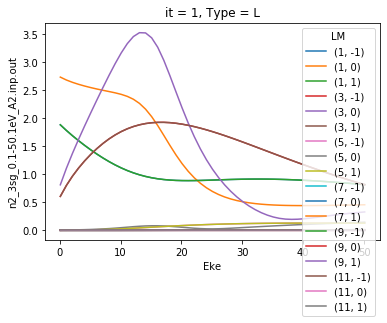
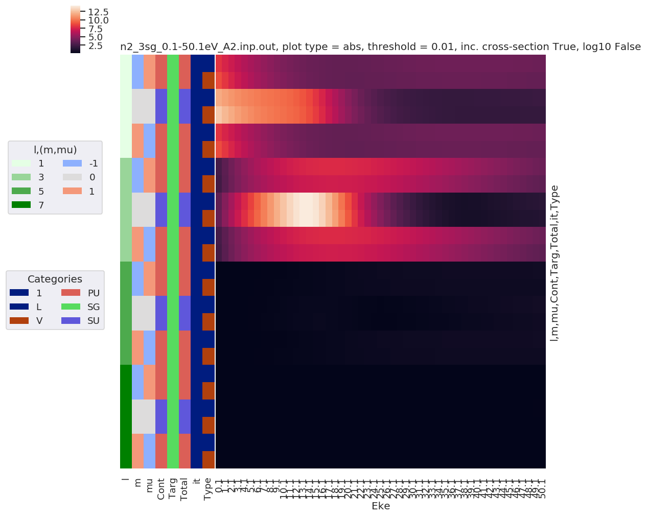
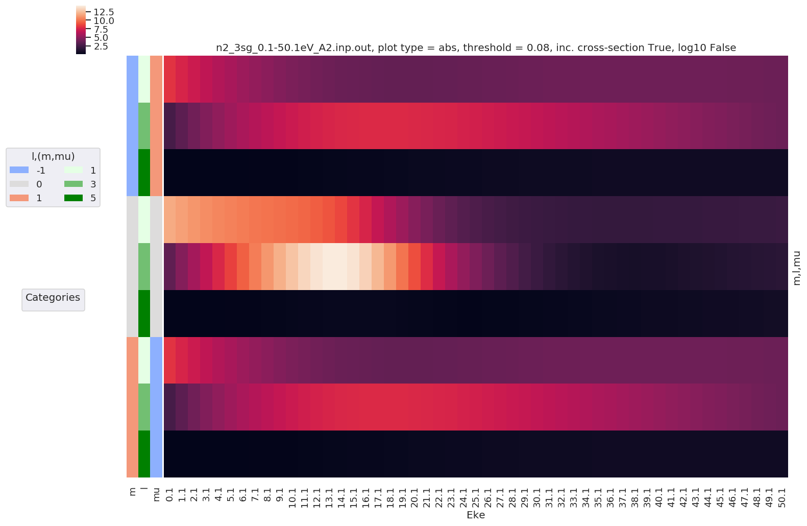
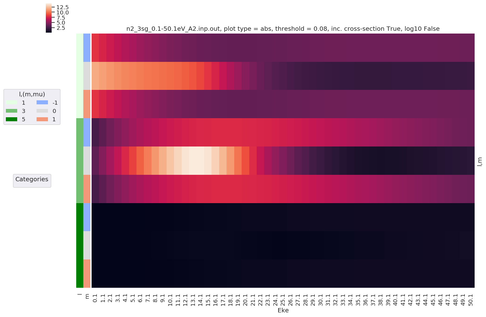
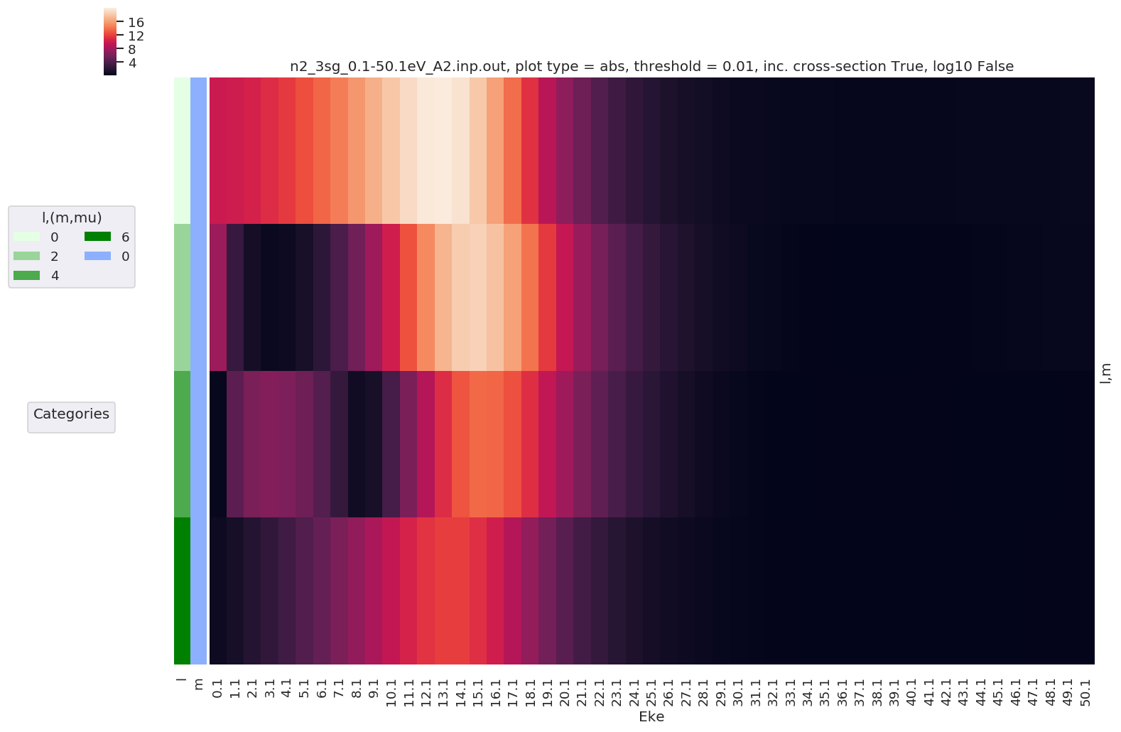
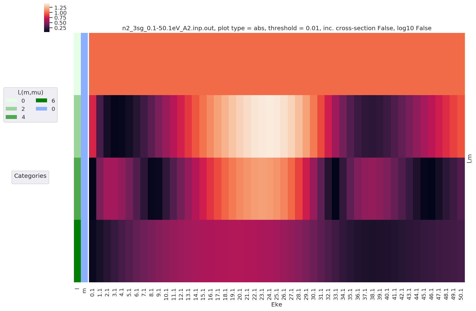
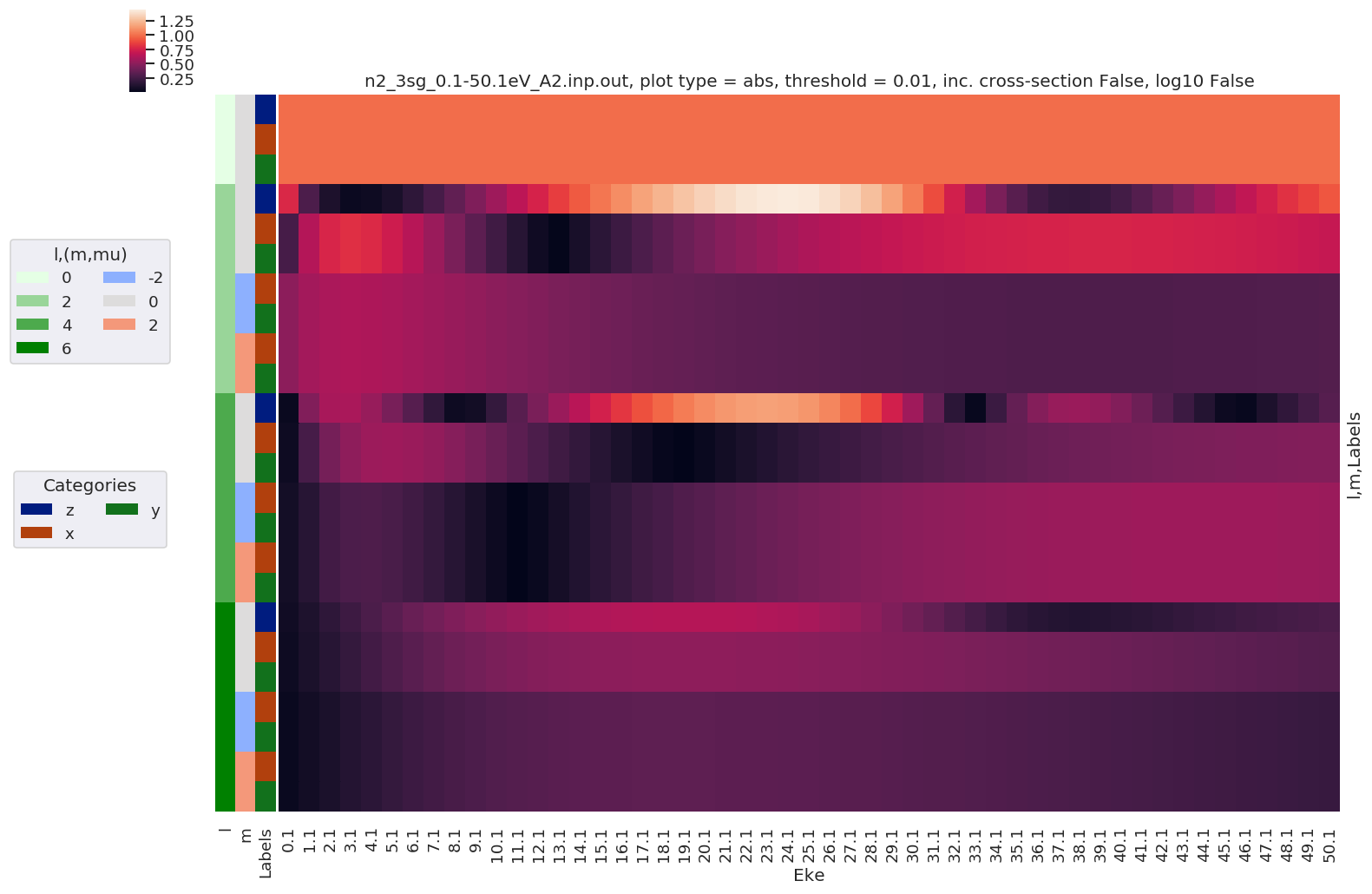
Plotting maps with lmPlot
For complex multidimensional cases line plots get busy, quickly. A nice alternative is provided by Seaborn’s Clustermap, which produces a 2D map of values (i.e. a heatmap or image), with additional dimensional information as a side-bar. This is now implemented in ep.lmPlot().
[8]:
# Plot with sensible defaults - all dims
daPlot, daPlotpd, legendList, gFig = ep.lmPlot(dataSet[0])
Plotting data n2_3sg_0.1-50.1eV_A2.inp.out, pType=a, thres=0.01, with Seaborn
In order to use Seaborn, the data is converted from a multidimensional Xarray to a 2D Pandas array. This displays nicely in Jupyter, so is also handy for inspecting values.
[9]:
daPlotpd
[9]:
| Eke | 0.1 | 1.1 | 2.1 | 3.1 | 4.1 | 5.1 | 6.1 | 7.1 | 8.1 | 9.1 | ... | 41.1 | 42.1 | 43.1 | 44.1 | 45.1 | 46.1 | 47.1 | 48.1 | 49.1 | 50.1 | |||||||
|---|---|---|---|---|---|---|---|---|---|---|---|---|---|---|---|---|---|---|---|---|---|---|---|---|---|---|---|---|
| l | m | mu | Cont | Targ | Total | it | Type | |||||||||||||||||||||
| 1 | -1 | 1 | PU | SG | PU | 1 | L | 8.143443 | 7.593716 | 7.103404 | 6.660060 | 6.255712 | 5.885550 | 5.546815 | 5.238038 | 4.958515 | 4.707928 | ... | 4.042680 | 4.036124 | 4.026955 | 4.015319 | 4.001367 | 3.985246 | 3.967107 | 3.947097 | 3.925361 | 3.902040 |
| V | 8.900023 | 8.224738 | 7.627702 | 7.095200 | 6.617558 | 6.187859 | 5.801034 | 5.453317 | 5.141863 | 4.864476 | ... | 3.819254 | 3.808920 | 3.796564 | 3.782339 | 3.766394 | 3.748875 | 3.729921 | 3.709668 | 3.688240 | 3.665757 | |||||||
| 0 | 0 | SU | SG | SU | 1 | L | 11.823354 | 11.429458 | 11.111935 | 10.849149 | 10.627257 | 10.437825 | 10.275304 | 10.134910 | 10.010680 | 9.893534 | ... | 2.013047 | 2.027855 | 2.044452 | 2.062457 | 2.081542 | 2.101424 | 2.121856 | 2.142623 | 2.163536 | 2.184431 | |
| V | 12.883046 | 12.311423 | 11.824577 | 11.410811 | 11.061133 | 10.768451 | 10.526367 | 10.328033 | 10.164873 | 10.025049 | ... | 1.911386 | 1.913114 | 1.917096 | 1.922952 | 1.930353 | 1.939023 | 1.948722 | 1.959246 | 1.970418 | 1.982089 | |||||||
| 1 | -1 | PU | SG | PU | 1 | L | 8.143443 | 7.593716 | 7.103404 | 6.660060 | 6.255712 | 5.885550 | 5.546815 | 5.238038 | 4.958515 | 4.707928 | ... | 4.042680 | 4.036124 | 4.026955 | 4.015319 | 4.001367 | 3.985246 | 3.967107 | 3.947097 | 3.925361 | 3.902040 | |
| V | 8.900023 | 8.224738 | 7.627702 | 7.095200 | 6.617558 | 6.187859 | 5.801034 | 5.453317 | 5.141863 | 4.864476 | ... | 3.819254 | 3.808920 | 3.796564 | 3.782339 | 3.766394 | 3.748875 | 3.729921 | 3.709668 | 3.688240 | 3.665757 | |||||||
| 3 | -1 | 1 | PU | SG | PU | 1 | L | 2.620714 | 3.416440 | 4.071325 | 4.629875 | 5.118714 | 5.553100 | 5.941282 | 6.287526 | 6.594077 | 6.862346 | ... | 5.148526 | 5.002561 | 4.857925 | 4.714821 | 4.573432 | 4.433917 | 4.296420 | 4.161067 | 4.027969 | 3.897223 |
| V | 2.484140 | 3.291182 | 3.949586 | 4.494447 | 4.953052 | 5.345025 | 5.683818 | 5.978440 | 6.234936 | 6.457456 | ... | 4.636261 | 4.495796 | 4.357692 | 4.222128 | 4.089249 | 3.959168 | 3.831972 | 3.707721 | 3.586455 | 3.468196 | |||||||
| 0 | 0 | SU | SG | SU | 1 | L | 3.513428 | 4.719556 | 5.785863 | 6.766306 | 7.695465 | 8.593950 | 9.472654 | 10.335015 | 11.177359 | 11.987428 | ... | 0.992670 | 1.058092 | 1.127714 | 1.198394 | 1.268089 | 1.335497 | 1.399805 | 1.460528 | 1.517392 | 1.570263 | |
| V | 3.682143 | 4.976274 | 6.086735 | 7.067816 | 7.963633 | 8.806609 | 9.618839 | 10.413320 | 11.194093 | 11.954877 | ... | 0.902085 | 0.948535 | 1.001878 | 1.058275 | 1.115154 | 1.170855 | 1.224342 | 1.274995 | 1.322471 | 1.366606 | |||||||
| 1 | -1 | PU | SG | PU | 1 | L | 2.620714 | 3.416440 | 4.071325 | 4.629875 | 5.118714 | 5.553100 | 5.941282 | 6.287526 | 6.594077 | 6.862346 | ... | 5.148526 | 5.002561 | 4.857925 | 4.714821 | 4.573432 | 4.433917 | 4.296420 | 4.161067 | 4.027969 | 3.897223 | |
| V | 2.484140 | 3.291182 | 3.949586 | 4.494447 | 4.953052 | 5.345025 | 5.683818 | 5.978440 | 6.234936 | 6.457456 | ... | 4.636261 | 4.495796 | 4.357692 | 4.222128 | 4.089249 | 3.959168 | 3.831972 | 3.707721 | 3.586455 | 3.468196 | |||||||
| 5 | -1 | 1 | PU | SG | PU | 1 | L | 0.003993 | 0.013835 | 0.021033 | 0.026999 | 0.033004 | 0.039974 | 0.048709 | 0.059861 | 0.073792 | 0.090524 | ... | 0.590336 | 0.593791 | 0.596895 | 0.599690 | 0.602218 | 0.604516 | 0.606620 | 0.608561 | 0.610372 | 0.612081 |
| V | 0.002819 | 0.010751 | 0.017869 | 0.026216 | 0.036675 | 0.049162 | 0.063460 | 0.079409 | 0.096872 | 0.115674 | ... | 0.525880 | 0.528078 | 0.530057 | 0.531856 | 0.533511 | 0.535057 | 0.536522 | 0.537936 | 0.539322 | 0.540704 | |||||||
| 0 | 0 | SU | SG | SU | 1 | L | 0.006473 | 0.021244 | 0.032261 | 0.041993 | 0.052580 | 0.065454 | 0.081763 | 0.102433 | 0.127951 | 0.158158 | ... | 0.498452 | 0.521782 | 0.544691 | 0.567177 | 0.589239 | 0.610871 | 0.632070 | 0.652828 | 0.673139 | 0.692996 | |
| V | 0.005091 | 0.017458 | 0.027707 | 0.039802 | 0.055471 | 0.074663 | 0.097135 | 0.122785 | 0.151483 | 0.182848 | ... | 0.407791 | 0.428275 | 0.448349 | 0.468019 | 0.487292 | 0.506174 | 0.524672 | 0.542791 | 0.560539 | 0.577920 | |||||||
| 1 | -1 | PU | SG | PU | 1 | L | 0.003993 | 0.013835 | 0.021033 | 0.026999 | 0.033004 | 0.039974 | 0.048709 | 0.059861 | 0.073792 | 0.090524 | ... | 0.590336 | 0.593791 | 0.596895 | 0.599690 | 0.602218 | 0.604516 | 0.606620 | 0.608561 | 0.610372 | 0.612081 | |
| V | 0.002819 | 0.010751 | 0.017869 | 0.026216 | 0.036675 | 0.049162 | 0.063460 | 0.079409 | 0.096872 | 0.115674 | ... | 0.525880 | 0.528078 | 0.530057 | 0.531856 | 0.533511 | 0.535057 | 0.536522 | 0.537936 | 0.539322 | 0.540704 | |||||||
| 7 | -1 | 1 | PU | SG | PU | 1 | L | 0.000024 | 0.000158 | 0.000305 | 0.000394 | 0.000405 | 0.000362 | 0.000320 | 0.000354 | 0.000491 | 0.000707 | ... | 0.031990 | 0.033121 | 0.034251 | 0.035381 | 0.036513 | 0.037648 | 0.038786 | 0.039930 | 0.041080 | 0.042237 |
| V | 0.000025 | 0.000150 | 0.000266 | 0.000318 | 0.000325 | 0.000356 | 0.000461 | 0.000630 | 0.000840 | 0.001086 | ... | 0.022021 | 0.022759 | 0.023500 | 0.024244 | 0.024994 | 0.025749 | 0.026511 | 0.027280 | 0.028058 | 0.028846 | |||||||
| 0 | 0 | SU | SG | SU | 1 | L | 0.000020 | 0.000145 | 0.000292 | 0.000373 | 0.000355 | 0.000266 | 0.000224 | 0.000373 | 0.000628 | 0.000955 | ... | 0.040133 | 0.042184 | 0.044257 | 0.046351 | 0.048466 | 0.050598 | 0.052748 | 0.054914 | 0.057094 | 0.059287 | |
| V | 0.000022 | 0.000137 | 0.000240 | 0.000265 | 0.000252 | 0.000340 | 0.000552 | 0.000822 | 0.001123 | 0.001465 | ... | 0.023763 | 0.025165 | 0.026594 | 0.028051 | 0.029534 | 0.031041 | 0.032572 | 0.034127 | 0.035704 | 0.037303 | |||||||
| 1 | -1 | PU | SG | PU | 1 | L | 0.000024 | 0.000158 | 0.000305 | 0.000394 | 0.000405 | 0.000362 | 0.000320 | 0.000354 | 0.000491 | 0.000707 | ... | 0.031990 | 0.033121 | 0.034251 | 0.035381 | 0.036513 | 0.037648 | 0.038786 | 0.039930 | 0.041080 | 0.042237 | |
| V | 0.000025 | 0.000150 | 0.000266 | 0.000318 | 0.000325 | 0.000356 | 0.000461 | 0.000630 | 0.000840 | 0.001086 | ... | 0.022021 | 0.022759 | 0.023500 | 0.024244 | 0.024994 | 0.025749 | 0.026511 | 0.027280 | 0.028058 | 0.028846 |
24 rows × 51 columns
[10]:
# With slicing by index (dims, energy)
daPlotpd.iloc[0:6, 0:6]
[10]:
| Eke | 0.1 | 1.1 | 2.1 | 3.1 | 4.1 | 5.1 | |||||||
|---|---|---|---|---|---|---|---|---|---|---|---|---|---|
| l | m | mu | Cont | Targ | Total | it | Type | ||||||
| 1 | -1 | 1 | PU | SG | PU | 1 | L | 8.143443 | 7.593716 | 7.103404 | 6.660060 | 6.255712 | 5.885550 |
| V | 8.900023 | 8.224738 | 7.627702 | 7.095200 | 6.617558 | 6.187859 | |||||||
| 0 | 0 | SU | SG | SU | 1 | L | 11.823354 | 11.429458 | 11.111935 | 10.849149 | 10.627257 | 10.437825 | |
| V | 12.883046 | 12.311423 | 11.824577 | 11.410811 | 11.061133 | 10.768451 | |||||||
| 1 | -1 | PU | SG | PU | 1 | L | 8.143443 | 7.593716 | 7.103404 | 6.660060 | 6.255712 | 5.885550 | |
| V | 8.900023 | 8.224738 | 7.627702 | 7.095200 | 6.617558 | 6.187859 |
Examples…
Various settings can be passed for more control over the plot.
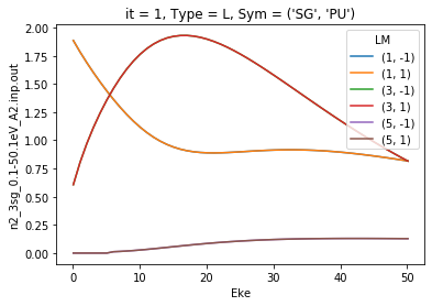
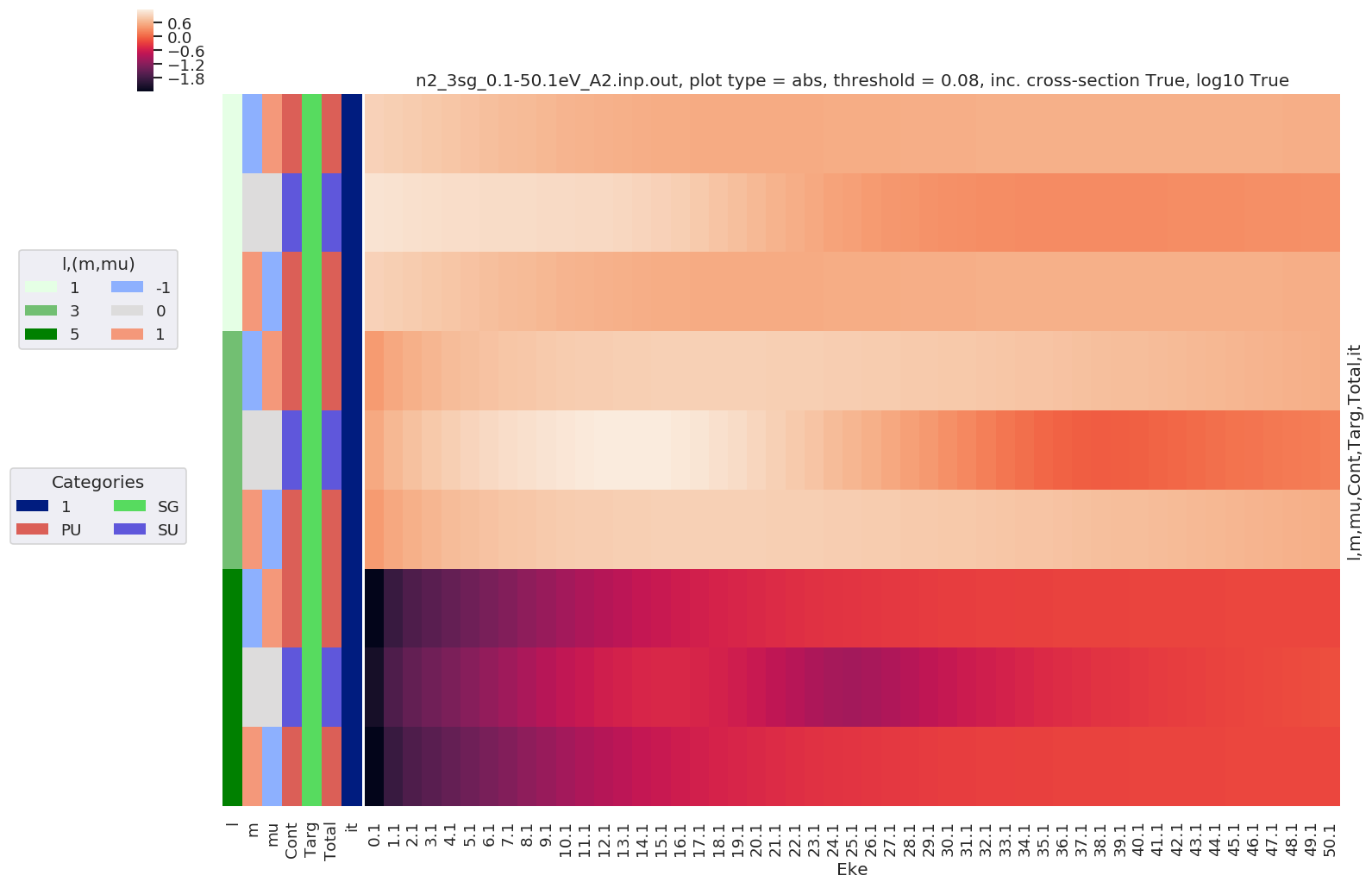
Example with - Selection on Type = L - Thresholding type by % of max value - Log10 scaling - Extended figure size
[11]:
daPlot, daPlotpd, legendList, gFig = ep.lmPlot(dataSet[0], selDims = {'Type':'L'},
                                               plotDims = ('l','m','mu','Cont','Targ','Total','it'),
                                               thresType='pc', thres = 0.01, figsize = (15,10), logFlag = True)
Plotting data n2_3sg_0.1-50.1eV_A2.inp.out, pType=a, thres=0.08224737585639882, with Seaborn
[12]:
daPlot.unstack().stack(plotDim = ('l','m','mu','Cont','Targ','Total'))
[12]:
<xarray.DataArray 'n2_3sg_0.1-50.1eV_A2.inp.out' (Eke: 51, it: 1, plotDim: 108)>
array([[[nan, nan, ..., nan, nan]],

       [[nan, nan, ..., nan, nan]],

       ...,

       [[nan, nan, ..., nan, nan]],

       [[nan, nan, ..., nan, nan]]])
Coordinates:
  * it       (it) int64 1
    Type     <U1 'L'
  * Eke      (Eke) float64 0.1 1.1 2.1 3.1 4.1 5.1 ... 46.1 47.1 48.1 49.1 50.1
    Ehv      (Eke) float64 15.68 16.68 17.68 18.68 ... 62.68 63.68 64.68 65.68
    SF       (Eke) complex128 (2.1560627+3.741674j) ... (4.4127053+1.8281945j)
  * plotDim  (plotDim) MultiIndex
  - l        (plotDim) int64 1 1 1 1 1 1 1 1 1 1 1 1 ... 5 5 5 5 5 5 5 5 5 5 5 5
  - m        (plotDim) int64 -1 -1 -1 -1 -1 -1 -1 -1 -1 -1 ... 1 1 1 1 1 1 1 1 1
  - mu       (plotDim) int64 -1 -1 -1 -1 0 0 0 0 1 1 1 ... -1 -1 0 0 0 0 1 1 1 1
  - Cont     (plotDim) object 'PU' 'PU' 'SU' 'SU' 'PU' ... 'PU' 'PU' 'SU' 'SU'
  - Targ     (plotDim) object 'SG' 'SG' 'SG' 'SG' 'SG' ... 'SG' 'SG' 'SG' 'SG'
  - Total    (plotDim) object 'PU' 'SU' 'PU' 'SU' 'PU' ... 'PU' 'SU' 'PU' 'SU'
Attributes:
    Lmax:          11
    Targ:          SG
    QNs:           ['m', 'l', 'mu', 'ip', 'it', 'Value']
    dataType:      matE
    file:          n2_3sg_0.1-50.1eV_A2.inp.out
    fileBase:      D:\code\github\ePSproc\data\photoionization
    pType:         a
    pTypeDetails:  {'Type': 'abs', 'Formula': 'np.abs(dataPlot)', 'Exec': <fu...
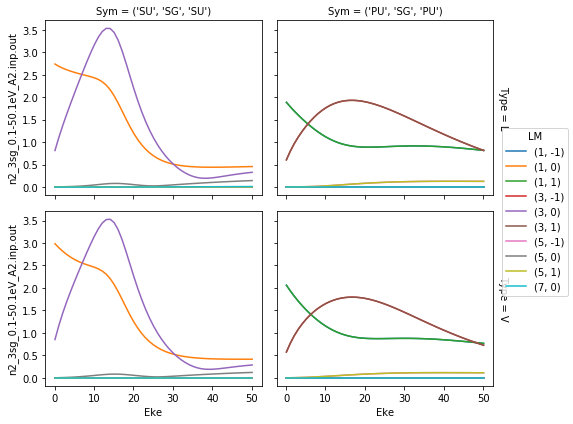
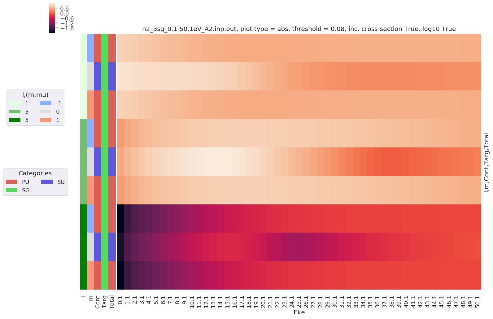
Example with - Selection on Type = L - Sum over mu - Thresholding type by % of max value - Log10 scaling - Extended figure size
[13]:
daPlot, daPlotpd, legendList, gFig = ep.lmPlot(dataSet[0], selDims = {'Type':'L'}, sumDims = ['mu'],
                                               plotDims = ('l','m','Cont','Targ','Total'),
                                               thresType='pc', thres = 0.01, figsize = (15,10), logFlag = True)
Plotting data n2_3sg_0.1-50.1eV_A2.inp.out, pType=a, thres=0.08224737585639882, with Seaborn
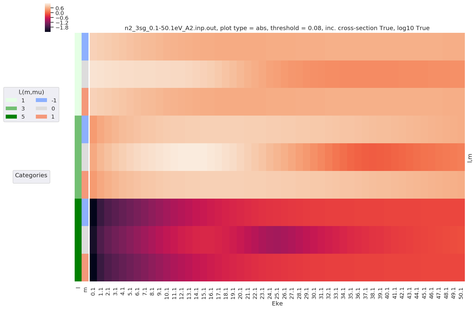
Example with - Selection on Type = L - Sum over mu and Sym - Thresholding type by % of max value - Log10 scaling - Extended figure size
[14]:
daPlot, daPlotpd, legendList, gFig = ep.lmPlot(dataSet[0], selDims = {'Type':'L'}, sumDims = ['mu', 'Sym'],
                                               plotDims = ('l','m'),
                                               thresType='pc', thres = 0.01, figsize = (15,10), logFlag = True)
Plotting data n2_3sg_0.1-50.1eV_A2.inp.out, pType=a, thres=0.08224737585639882, with Seaborn
No handles with labels found to put in legend.
Example with - Changing the ordering of plotDims, here with ‘m’ as the main index.
[15]:
daPlot, daPlotpd, legendList, gFig = ep.lmPlot(dataSet[0], selDims = {'Type':'L'}, sumDims = ['Sym'],
                                               plotDims = ('m','l','mu'),
                                               thresType='pc', thres = 0.01, figsize = (15,10))
Plotting data n2_3sg_0.1-50.1eV_A2.inp.out, pType=a, thres=0.08224737585639882, with Seaborn
No handles with labels found to put in legend.
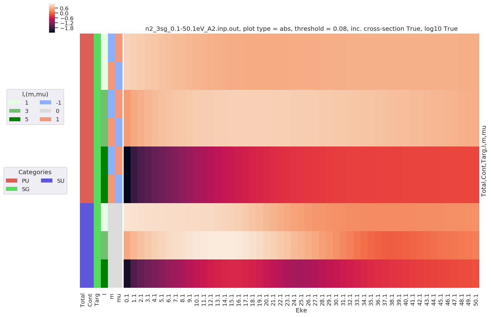
Example with - Ordering by symmetry group.
[16]:
daPlot, daPlotpd, legendList, gFig = ep.lmPlot(dataSet[0], selDims = {'Type':'L'},
                                               plotDims = ('Total','Cont','Targ','l','m','mu'),
                                               thresType='pc', thres = 0.01, figsize = (15,10), logFlag = True)
Plotting data n2_3sg_0.1-50.1eV_A2.inp.out, pType=a, thres=0.08224737585639882, with Seaborn
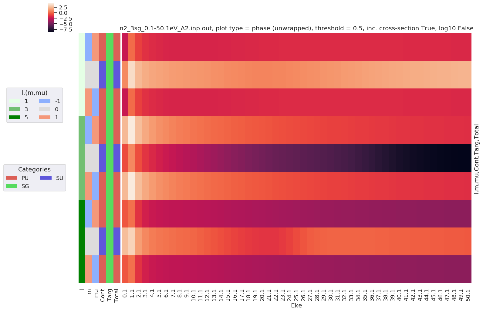
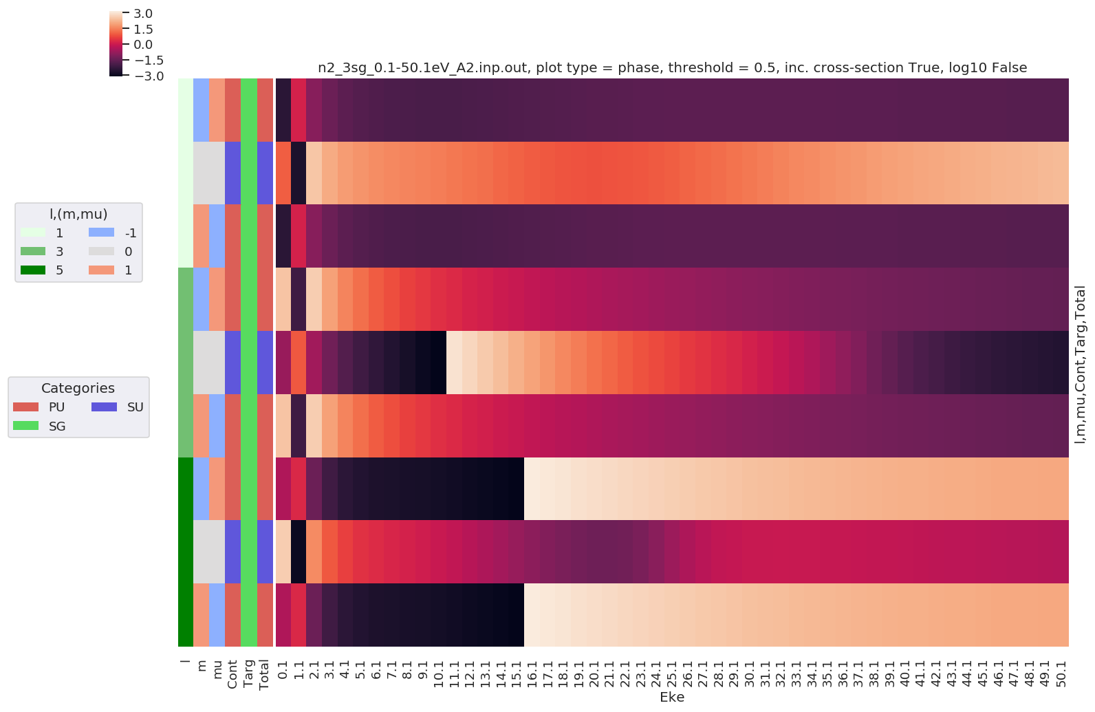
Example with - Unwrapped phase plot
[17]:
daPlot, daPlotpd, legendList, gFig = ep.lmPlot(dataSet[0], selDims = {'Type':'L'},
                                               plotDims = ('l','m','mu','Cont','Targ','Total'),
                                               thres = 0.5, figsize = (15,10),
                                               pType = 'phaseUW')
C:\Program Files (x86)\Microsoft Visual Studio\Shared\Anaconda3_64\envs\ePSdev\lib\site-packages\numpy\lib\function_base.py:1519: RuntimeWarning:

invalid value encountered in remainder

C:\Program Files (x86)\Microsoft Visual Studio\Shared\Anaconda3_64\envs\ePSdev\lib\site-packages\numpy\lib\function_base.py:1520: RuntimeWarning:

invalid value encountered in greater

C:\Program Files (x86)\Microsoft Visual Studio\Shared\Anaconda3_64\envs\ePSdev\lib\site-packages\numpy\lib\function_base.py:1522: RuntimeWarning:

invalid value encountered in less
Plotting data n2_3sg_0.1-50.1eV_A2.inp.out, pType=phaseUW, thres=0.5, with Seaborn
Further analysis examples
Summations
- Sum over Eke, plot by l.
[18]:
daPlot, daPlotpd, legendList, gFig = ep.lmPlot(dataSet[0], selDims = {'Type':'L'}, xDim = 'LM', sumDims = 'Eke',
                                               plotDims = ('Total','Cont','Targ','m','mu'),
                                               thresType='pc', thres = 0.01, figsize = (15,10),
                                               cmap = 'Greens')
Plotting data n2_3sg_0.1-50.1eV_A2.inp.out, pType=a, thres=0.08224737585639882, with Seaborn
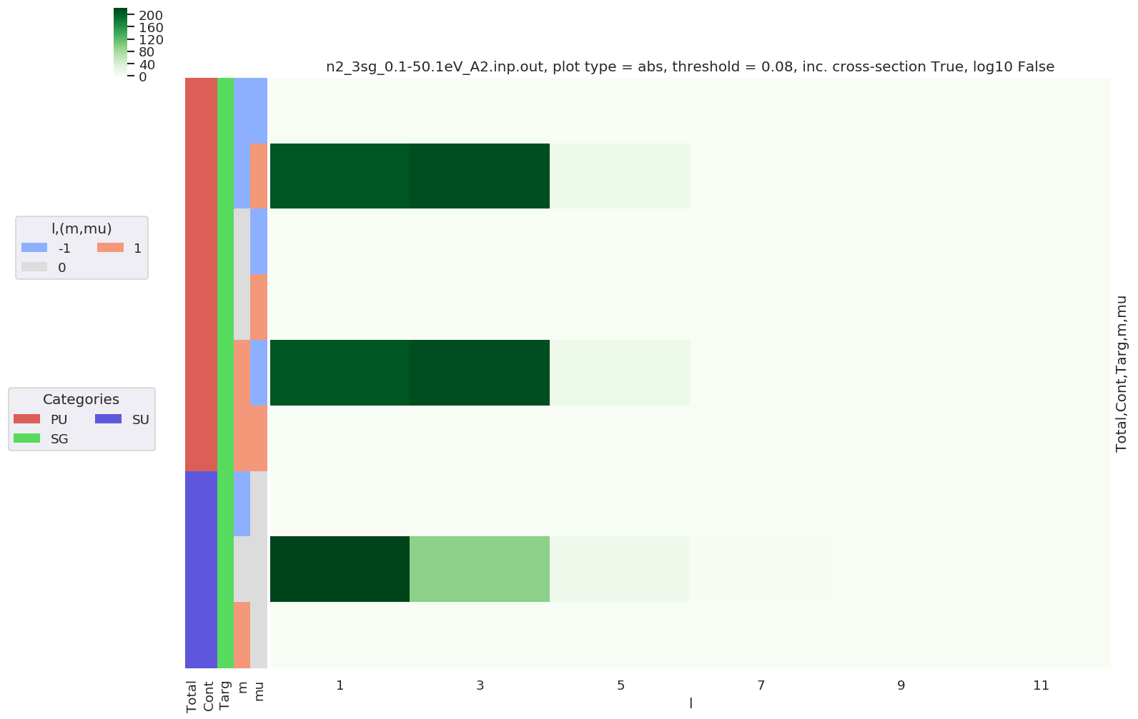
[19]:
daPlotpd
[19]:
| l | 1 | 3 | 5 | 7 | 9 | 11 | ||||
|---|---|---|---|---|---|---|---|---|---|---|
| Total | Cont | Targ | m | mu | ||||||
| PU | PU | SG | -1 | -1 | 0.000000 | 0.000000 | 0.000000 | 0.000000 | 0.000000 | 0.000000 |
| 1 | 207.905550 | 212.622228 | 17.570951 | 0.779478 | 0.020871 | 0.000572 | ||||
| 0 | -1 | 0.000000 | 0.000000 | 0.000000 | 0.000000 | 0.000000 | 0.000000 | |||
| 1 | 0.000000 | 0.000000 | 0.000000 | 0.000000 | 0.000000 | 0.000000 | ||||
| 1 | -1 | 207.905550 | 212.622228 | 17.570951 | 0.779478 | 0.020871 | 0.000572 | |||
| 1 | 0.000000 | 0.000000 | 0.000000 | 0.000000 | 0.000000 | 0.000000 | ||||
| SU | SU | SG | -1 | 0 | 0.000000 | 0.000000 | 0.000000 | 0.000000 | 0.000000 | 0.000000 |
| 0 | 0 | 220.297545 | 95.032282 | 13.737638 | 0.950270 | 0.026699 | 0.000313 | |||
| 1 | 0 | 0.000000 | 0.000000 | 0.000000 | 0.000000 | 0.000000 | 0.000000 |
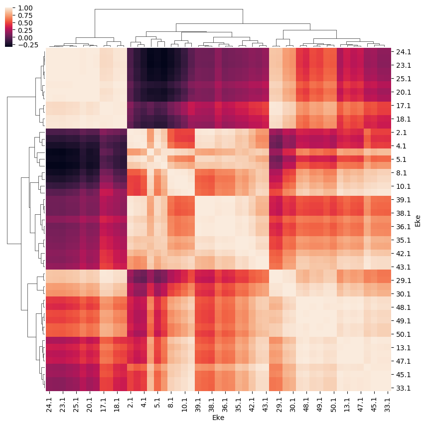
Correlations
- Correlation plots from the Pandas representation with
`pandas.corr()<https://pandas.pydata.org/pandas-docs/stable/user_guide/computation.html#correlation>`__. This defaults to a Pearson correlation coefficient, but other types of correlation functions can be used. Work in progress!
[20]:
ep.snsMatMod.clustermap(daPlotpd.corr())
[20]:
<epsproc._sns_matrixMod.ClusterGrid at 0x229ffcb6908>
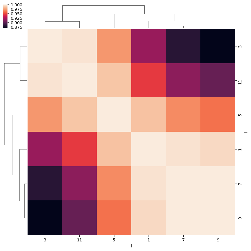
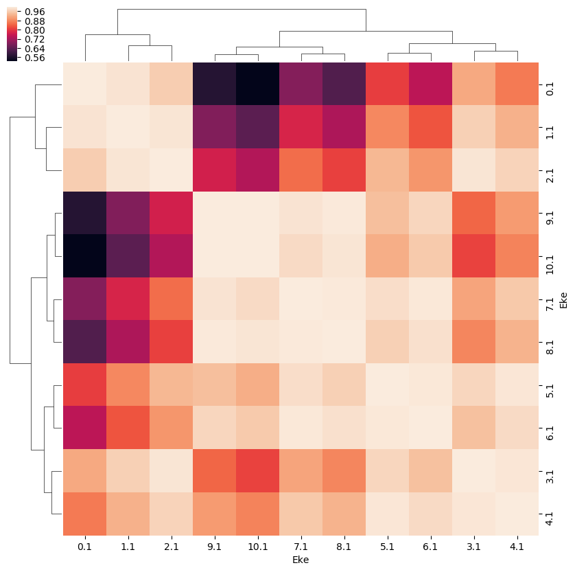
- Sum over symetries, plot by Eke.
[21]:
daPlot, daPlotpd, legendList, gFig = ep.lmPlot(dataSet[0], selDims = {'Type':'L'}, sumDims = ['mu', 'Sym'],
                                               plotDims = ('l','m'),
                                               thresType='pc', thres = 0.01, figsize = (15,10))
Plotting data n2_3sg_0.1-50.1eV_A2.inp.out, pType=a, thres=0.08224737585639882, with Seaborn
No handles with labels found to put in legend.
[22]:
# Display values for first 10 Ekes
daPlotpd.iloc[:,0:11]
[22]:
| Eke | 0.1 | 1.1 | 2.1 | 3.1 | 4.1 | 5.1 | 6.1 | 7.1 | 8.1 | 9.1 | 10.1 | |
|---|---|---|---|---|---|---|---|---|---|---|---|---|
| l | m | |||||||||||
| 1 | -1 | 8.143443 | 7.593716 | 7.103404 | 6.660060 | 6.255712 | 5.885550 | 5.546815 | 5.238038 | 4.958515 | 4.707928 | 4.486077 |
| 0 | 11.823354 | 11.429458 | 11.111935 | 10.849149 | 10.627257 | 10.437825 | 10.275304 | 10.134910 | 10.010680 | 9.893534 | 9.769350 | |
| 1 | 8.143443 | 7.593716 | 7.103404 | 6.660060 | 6.255712 | 5.885550 | 5.546815 | 5.238038 | 4.958515 | 4.707928 | 4.486077 | |
| 3 | -1 | 2.620714 | 3.416440 | 4.071325 | 4.629875 | 5.118714 | 5.553100 | 5.941282 | 6.287526 | 6.594077 | 6.862346 | 7.093572 |
| 0 | 3.513428 | 4.719556 | 5.785863 | 6.766306 | 7.695465 | 8.593950 | 9.472654 | 10.335015 | 11.177359 | 11.987428 | 12.741400 | |
| 1 | 2.620714 | 3.416440 | 4.071325 | 4.629875 | 5.118714 | 5.553100 | 5.941282 | 6.287526 | 6.594077 | 6.862346 | 7.093572 | |
| 5 | -1 | 0.003993 | 0.013835 | 0.021033 | 0.026999 | 0.033004 | 0.039974 | 0.048709 | 0.059861 | 0.073792 | 0.090524 | 0.109801 |
| 0 | 0.006473 | 0.021244 | 0.032261 | 0.041993 | 0.052580 | 0.065454 | 0.081763 | 0.102433 | 0.127951 | 0.158158 | 0.192134 | |
| 1 | 0.003993 | 0.013835 | 0.021033 | 0.026999 | 0.033004 | 0.039974 | 0.048709 | 0.059861 | 0.073792 | 0.090524 | 0.109801 |
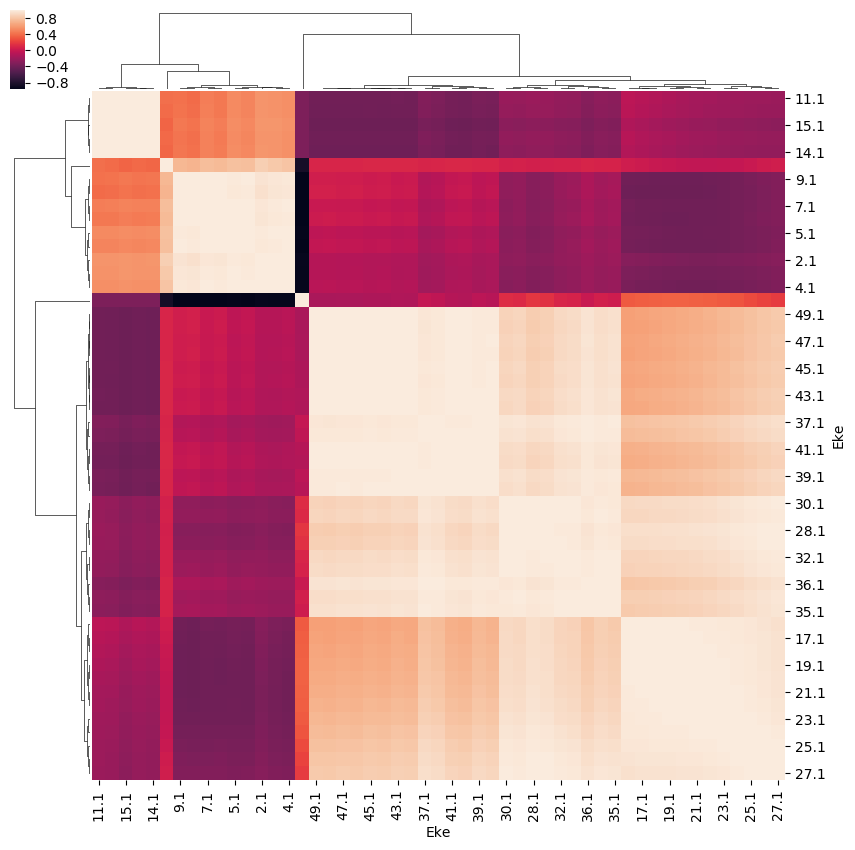
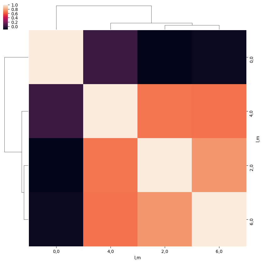
- Correlations…
[23]:
# Eke correlations
ep.snsMatMod.clustermap(daPlotpd.iloc[:,0:11].corr())
[23]:
<epsproc._sns_matrixMod.ClusterGrid at 0x229ffc27d68>
[24]:
# (l,m) correlations
ep.snsMatMod.clustermap(daPlotpd.iloc[:,0:11].T.corr())
[24]:
<epsproc._sns_matrixMod.ClusterGrid at 0x229f9b9c9e8>
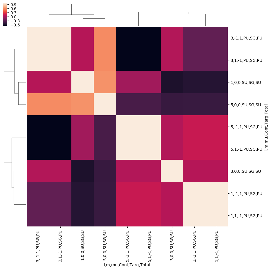
Phase correlations
- Full phases and correlations…
[25]:
daPlot, daPlotpd, legendList, gFig = ep.lmPlot(dataSet[0], selDims = {'Type':'L'},
                                               plotDims = ('l','m','mu','Cont','Targ','Total'),
                                               thres = 0.5, figsize = (15,10),
                                               pType = 'phase')
Plotting data n2_3sg_0.1-50.1eV_A2.inp.out, pType=phase, thres=0.5, with Seaborn
[26]:
# ep.snsMatMod.clustermap(daPlotpd.iloc[:,0:11].corr())
ep.snsMatMod.clustermap(daPlotpd.corr())
[26]:
<epsproc._sns_matrixMod.ClusterGrid at 0x229fc665e48>
[27]:
# ep.snsMatMod.clustermap(daPlotpd.iloc[:,0:11].T.corr())
ep.snsMatMod.clustermap(daPlotpd.T.corr())
[27]:
<epsproc._sns_matrixMod.ClusterGrid at 0x229ffe65f60>
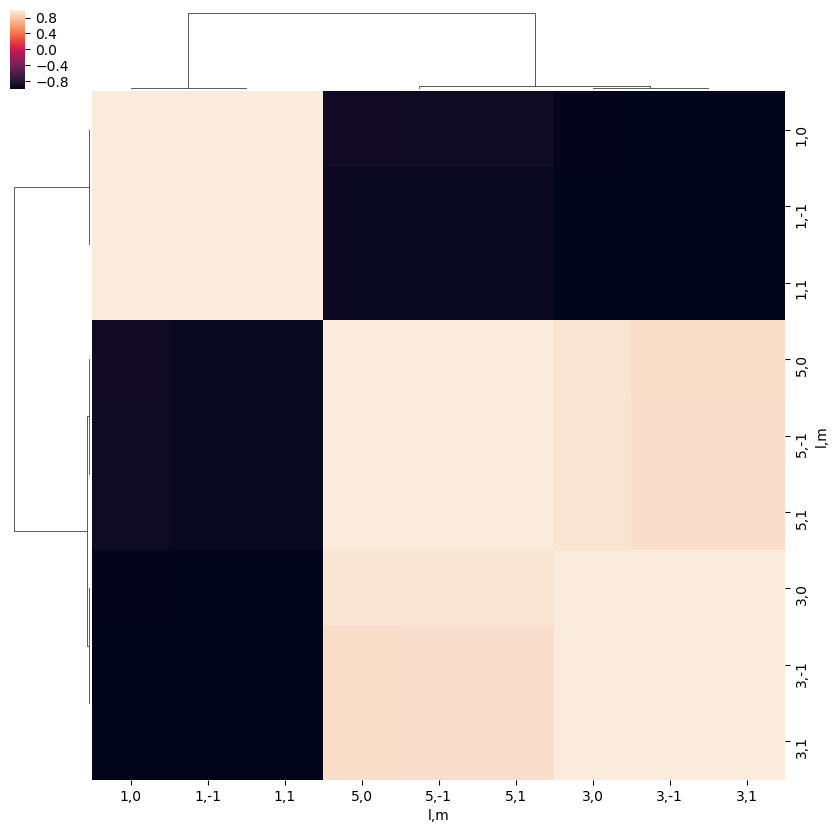
For \(\beta_{L,M}\)
The same functionality can be applied to plotting \(\beta_{L,M}\) paramters…
(For calculation details, see :math:beta_{L,M}` calculations demo notebook <https://github.com/phockett/ePSproc/blob/master/epsproc/tests/ePSproc_BLM_calc_demo_Sept2019.ipynb>`__.)
[28]:
daIn = dataSet[0].copy()
BLMXeN2 = ep.mfblm(daIn, selDims = {'Type':'L'}, thres = 1e-2, verbose = 0)   # Run for all Eke
[29]:
daPlot, daPlotpd, legendList, gFig = ep.lmPlot(BLMXeN2, SFflag = True,
                                               plotDims = ('l','m'), sumDims = ('Euler'),
                                               figsize = (15,10))
Plotting data n2_3sg_0.1-50.1eV_A2.inp.out, pType=a, thres=0.01, with Seaborn
No handles with labels found to put in legend.
- \(\beta_{L,M}\) correlations over Eke
[30]:
ep.snsMatMod.clustermap(daPlotpd.corr())
[30]:
<epsproc._sns_matrixMod.ClusterGrid at 0x22983bfd2b0>
For the \(\beta_{L,M}\) case, the SFflag controls whether normalised or unnormalised values are plotted. In the former case, the cross-section (\(\beta_{0,0}\)) is divided out, hence \(\beta_{0,0}\) = 1.
[31]:
daPlot, daPlotpd, legendList, gFig = ep.lmPlot(BLMXeN2, SFflag = False,
                                               plotDims = ('l','m'),
                                               figsize = (15,10))
Plotting data n2_3sg_0.1-50.1eV_A2.inp.out, pType=a, thres=0.01, with Seaborn
No handles with labels found to put in legend.
[32]:
ep.snsMatMod.clustermap(daPlotpd.T.corr())
[32]:
<epsproc._sns_matrixMod.ClusterGrid at 0x229ffa9ceb8>
As a function of Euler angle…
[33]:
# Set pol geoms - these correspond to (z,x,y) in molecular frame (relative to principle/symmetry axis)
# pRot = [0, 0, np.pi/2]
# tRot = [0, np.pi/2, np.pi/2]
# cRot = [0, 0, 0]
# eAngs = np.array([pRot, tRot, cRot]).T   # List form to use later, rows per set of angles

eAngs = ep.setPolGeoms()  # Functionalised form, returns Xarray of pol geoms, defaults to (z,x,y)
[34]:
thres = 1e-2
# Calculate for each pol geom
# Run for all Eke, selected gauge only; round angles for display purposes only (to be fixed!)
BLMeuler = ep.mfblmEuler(daIn, selDims = {'Type':'L'}, eAngs = eAngs, thres = thres, verbose = 0)
BLMeulerLabel = BLMeuler.drop('Euler').swap_dims({'Euler':'Labels'})  # Swap values and labels for plotting, otherwise will be plotted vs. Euler angles
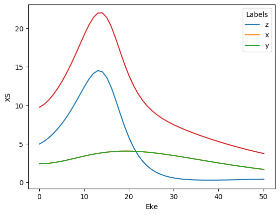
Cross-sections…
[35]:
# Check XS values
BLMeulerLabel.XS.real.plot.line(x='Eke');
# BLMeuler.XS.sum('Euler').real.plot.line(x='Eke');  # Add sum over Euler angles sets
BLMeulerLabel.XS.sum('Labels').real.plot.line(x='Eke');  # Add sum over Euler angles sets
C:\Program Files (x86)\Microsoft Visual Studio\Shared\Anaconda3_64\envs\ePSdev\lib\site-packages\xarray\plot\plot.py:76: FutureWarning:

This DataArray contains multi-dimensional coordinates. In the future, these coordinates will be transposed as well unless you specify transpose_coords=False.
[36]:
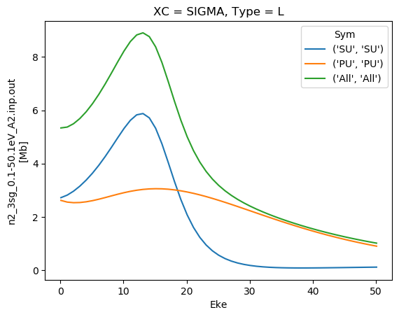
# Check XS from ePS file GetCRO outputs
# This is for each symmetry group, averaged over all angles (i.e. unaligned LF) - see ePS manaul, https://www.chem.tamu.edu/rgroup/lucchese/ePolyScat.E3.manual/GetCro.html
# Hence should be similar to (x,y,z) MF orientations, but not identical
dataXS[0].sel({'XC':'SIGMA', 'Type':'L'}).plot.line(x='Eke');
\(\beta_{L,M}\) parameters…
[37]:
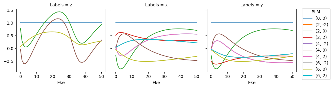
# Plot (normalised) BLM results - basic with Xarray (note Seaborn style may now be applied, since lmPlot() sets this globally)
BLMplot = ep.matEleSelector(BLMeulerLabel, thres=thres, dims = 'Eke')
BLMplot.real.squeeze().plot.line(x='Eke', col='Labels');
[38]:
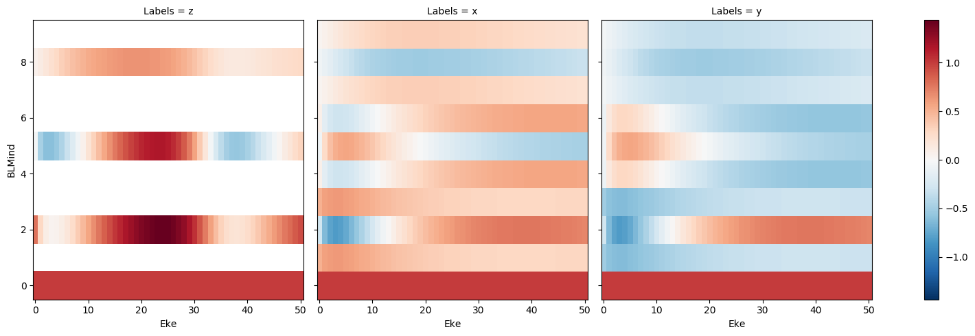
# Plot resutls - 2D maps with Xarray, faceted on Euler angle sets
# Set BLM index for y-axis
BLMplot['BLMind'] = ('BLM',np.arange(0, BLMplot.BLM.size))
# Plot
BLMplot.real.squeeze().plot(x='Eke', y='BLMind', col='Labels', size = 5);
[39]:
# Plot results with lmPlot()
daPlot, daPlotpd, legendList, gFig = ep.lmPlot(BLMeuler, SFflag = False, eulerGroup = True,
                                               plotDims = ('l','m','Labels'),
                                               figsize = (15,10))
Plotting data n2_3sg_0.1-50.1eV_A2.inp.out, pType=a, thres=0.01, with Seaborn
[40]:
daPlotpd
[40]:
| Eke | 0.1 | 1.1 | 2.1 | 3.1 | 4.1 | 5.1 | 6.1 | 7.1 | 8.1 | 9.1 | ... | 41.1 | 42.1 | 43.1 | 44.1 | 45.1 | 46.1 | 47.1 | 48.1 | 49.1 | 50.1 | ||
|---|---|---|---|---|---|---|---|---|---|---|---|---|---|---|---|---|---|---|---|---|---|---|---|
| l | m | Labels | |||||||||||||||||||||
| 0 | 0 | z | 1.000000 | 1.000000 | 1.000000 | 1.000000 | 1.000000 | 1.000000 | 1.000000 | 1.000000 | 1.000000 | 1.000000 | ... | 1.000000 | 1.000000 | 1.000000 | 1.000000 | 1.000000 | 1.000000 | 1.000000 | 1.000000 | 1.000000 | 1.000000 |
| x | 1.000000 | 1.000000 | 1.000000 | 1.000000 | 1.000000 | 1.000000 | 1.000000 | 1.000000 | 1.000000 | 1.000000 | ... | 1.000000 | 1.000000 | 1.000000 | 1.000000 | 1.000000 | 1.000000 | 1.000000 | 1.000000 | 1.000000 | 1.000000 | ||
| y | 1.000000 | 1.000000 | 1.000000 | 1.000000 | 1.000000 | 1.000000 | 1.000000 | 1.000000 | 1.000000 | 1.000000 | ... | 1.000000 | 1.000000 | 1.000000 | 1.000000 | 1.000000 | 1.000000 | 1.000000 | 1.000000 | 1.000000 | 1.000000 | ||
| 2 | 0 | z | 0.785011 | 0.293449 | 0.111540 | 0.049561 | 0.056243 | 0.104724 | 0.178871 | 0.268287 | 0.365983 | 0.467176 | ... | 0.320748 | 0.389800 | 0.463637 | 0.538792 | 0.612895 | 0.684425 | 0.752480 | 0.816588 | 0.876568 | 0.932425 |
| x | 0.272486 | 0.637673 | 0.773735 | 0.812507 | 0.791447 | 0.732312 | 0.649701 | 0.553911 | 0.452233 | 0.349699 | ... | 0.764359 | 0.761156 | 0.756929 | 0.751725 | 0.745586 | 0.738551 | 0.730656 | 0.721932 | 0.712410 | 0.702118 | ||
| y | 0.272486 | 0.637673 | 0.773735 | 0.812507 | 0.791447 | 0.732312 | 0.649701 | 0.553911 | 0.452233 | 0.349699 | ... | 0.764359 | 0.761156 | 0.756929 | 0.751725 | 0.745586 | 0.738551 | 0.730656 | 0.721932 | 0.712410 | 0.702118 | ||
| -2 | x | 0.512057 | 0.586600 | 0.614373 | 0.622288 | 0.617989 | 0.605918 | 0.589055 | 0.569502 | 0.548747 | 0.527818 | ... | 0.300411 | 0.301065 | 0.301928 | 0.302990 | 0.304243 | 0.305679 | 0.307291 | 0.309072 | 0.311015 | 0.313116 | |
| y | 0.512057 | 0.586600 | 0.614373 | 0.622288 | 0.617989 | 0.605918 | 0.589055 | 0.569502 | 0.548747 | 0.527818 | ... | 0.300411 | 0.301065 | 0.301928 | 0.302990 | 0.304243 | 0.305679 | 0.307291 | 0.309072 | 0.311015 | 0.313116 | ||
| 2 | x | 0.512057 | 0.586600 | 0.614373 | 0.622288 | 0.617989 | 0.605918 | 0.589055 | 0.569502 | 0.548747 | 0.527818 | ... | 0.300411 | 0.301065 | 0.301928 | 0.302990 | 0.304243 | 0.305679 | 0.307291 | 0.309072 | 0.311015 | 0.313116 | |
| y | 0.512057 | 0.586600 | 0.614373 | 0.622288 | 0.617989 | 0.605918 | 0.589055 | 0.569502 | 0.548747 | 0.527818 | ... | 0.300411 | 0.301065 | 0.301928 | 0.302990 | 0.304243 | 0.305679 | 0.307291 | 0.309072 | 0.311015 | 0.313116 | ||
| 4 | 0 | z | 0.040440 | 0.474638 | 0.598502 | 0.603911 | 0.543444 | 0.444731 | 0.324406 | 0.193160 | 0.058087 | 0.076090 | ... | 0.405478 | 0.321374 | 0.231758 | 0.140971 | 0.051947 | 0.033463 | 0.114184 | 0.189684 | 0.259784 | 0.324538 |
| x | 0.059137 | 0.269489 | 0.430702 | 0.519099 | 0.560386 | 0.569288 | 0.555695 | 0.526731 | 0.487676 | 0.442441 | ... | 0.434418 | 0.441791 | 0.448488 | 0.454535 | 0.459955 | 0.464771 | 0.469002 | 0.472664 | 0.475772 | 0.478341 | ||
| y | 0.059137 | 0.269489 | 0.430702 | 0.519099 | 0.560386 | 0.569288 | 0.555695 | 0.526731 | 0.487676 | 0.442441 | ... | 0.434418 | 0.441791 | 0.448488 | 0.454535 | 0.459955 | 0.464771 | 0.469002 | 0.472664 | 0.475772 | 0.478341 | ||
| -2 | x | 0.080476 | 0.152557 | 0.251643 | 0.293304 | 0.298915 | 0.280822 | 0.247316 | 0.204290 | 0.155991 | 0.105436 | ... | 0.565731 | 0.566930 | 0.567553 | 0.567625 | 0.567169 | 0.566205 | 0.564751 | 0.562825 | 0.560441 | 0.557615 | |
| y | 0.080476 | 0.152557 | 0.251643 | 0.293304 | 0.298915 | 0.280822 | 0.247316 | 0.204290 | 0.155991 | 0.105436 | ... | 0.565731 | 0.566930 | 0.567553 | 0.567625 | 0.567169 | 0.566205 | 0.564751 | 0.562825 | 0.560441 | 0.557615 | ||
| 2 | x | 0.080476 | 0.152557 | 0.251643 | 0.293304 | 0.298915 | 0.280822 | 0.247316 | 0.204290 | 0.155991 | 0.105436 | ... | 0.565731 | 0.566930 | 0.567553 | 0.567625 | 0.567169 | 0.566205 | 0.564751 | 0.562825 | 0.560441 | 0.557615 | |
| y | 0.080476 | 0.152557 | 0.251643 | 0.293304 | 0.298915 | 0.280822 | 0.247316 | 0.204290 | 0.155991 | 0.105436 | ... | 0.565731 | 0.566930 | 0.567553 | 0.567625 | 0.567169 | 0.566205 | 0.564751 | 0.562825 | 0.560441 | 0.557615 | ||
| 6 | 0 | z | 0.068194 | 0.122431 | 0.179261 | 0.235361 | 0.289105 | 0.339558 | 0.386124 | 0.428443 | 0.466366 | 0.499925 | ... | 0.164395 | 0.179851 | 0.196062 | 0.212134 | 0.227491 | 0.241791 | 0.254860 | 0.266630 | 0.277105 | 0.286334 |
| x | 0.059156 | 0.106111 | 0.155866 | 0.205371 | 0.252784 | 0.296866 | 0.336789 | 0.372096 | 0.402658 | 0.428609 | ... | 0.389928 | 0.381806 | 0.373613 | 0.365354 | 0.357037 | 0.348667 | 0.340251 | 0.331793 | 0.323301 | 0.314781 | ||
| y | 0.059156 | 0.106111 | 0.155866 | 0.205371 | 0.252784 | 0.296866 | 0.336789 | 0.372096 | 0.402658 | 0.428609 | ... | 0.389928 | 0.381806 | 0.373613 | 0.365354 | 0.357037 | 0.348667 | 0.340251 | 0.331793 | 0.323301 | 0.314781 | ||
| -2 | x | 0.040411 | 0.072488 | 0.106477 | 0.140295 | 0.172685 | 0.202798 | 0.230071 | 0.254190 | 0.275068 | 0.292796 | ... | 0.266372 | 0.260823 | 0.255226 | 0.249585 | 0.243903 | 0.238185 | 0.232435 | 0.226658 | 0.220857 | 0.215037 | |
| y | 0.040411 | 0.072488 | 0.106477 | 0.140295 | 0.172685 | 0.202798 | 0.230071 | 0.254190 | 0.275068 | 0.292796 | ... | 0.266372 | 0.260823 | 0.255226 | 0.249585 | 0.243903 | 0.238185 | 0.232435 | 0.226658 | 0.220857 | 0.215037 | ||
| 2 | x | 0.040411 | 0.072488 | 0.106477 | 0.140295 | 0.172685 | 0.202798 | 0.230071 | 0.254190 | 0.275068 | 0.292796 | ... | 0.266372 | 0.260823 | 0.255226 | 0.249585 | 0.243903 | 0.238185 | 0.232435 | 0.226658 | 0.220857 | 0.215037 | |
| y | 0.040411 | 0.072488 | 0.106477 | 0.140295 | 0.172685 | 0.202798 | 0.230071 | 0.254190 | 0.275068 | 0.292796 | ... | 0.266372 | 0.260823 | 0.255226 | 0.249585 | 0.243903 | 0.238185 | 0.232435 | 0.226658 | 0.220857 | 0.215037 |
24 rows × 51 columns
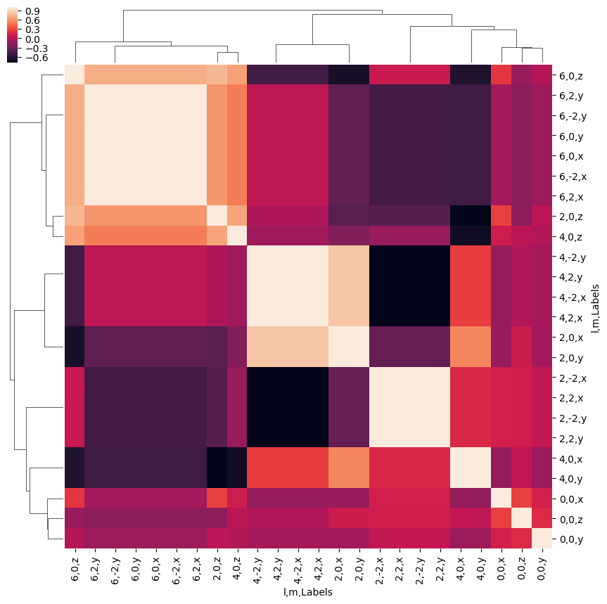
- Look at correlations over all (l,m,Euler)
[41]:
ep.snsMatMod.clustermap(daPlotpd.T.corr())
[41]:
<epsproc._sns_matrixMod.ClusterGrid at 0x2298740d6a0>
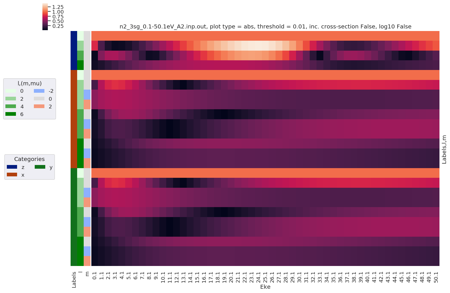
- Replot with sorting by Euler sets
[42]:
# Plot results with lmPlot(), ordering by Euler sets
daPlot, daPlotpd, legendList, gFig = ep.lmPlot(BLMeuler, SFflag = False, eulerGroup = True,
                                               plotDims = ('Labels','l','m'),
                                               figsize = (15,10))
Plotting data n2_3sg_0.1-50.1eV_A2.inp.out, pType=a, thres=0.01, with Seaborn
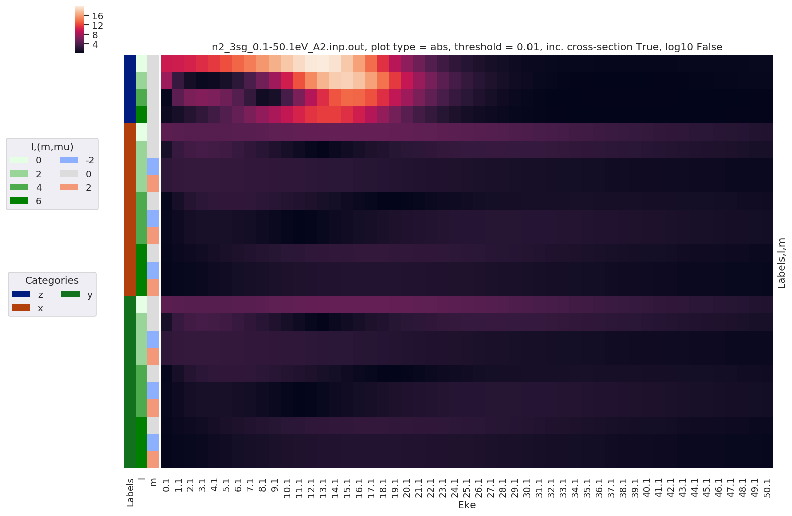
… and including cross-section …
[43]:
# Plot results with lmPlot(), ordering by Euler sets + use XS
# NOTE - this currently plots with unstacked Euler angles (P,T,C) - should change to treat these as a stacked set.
daPlot, daPlotpd, legendList, gFig = ep.lmPlot(BLMeuler, SFflag = True,
                                               plotDims = ('Labels','l','m'),
                                               figsize = (15,10))
Plotting data n2_3sg_0.1-50.1eV_A2.inp.out, pType=a, thres=0.01, with Seaborn
[44]:
daPlotpd
[44]:
| Eke | 0.1 | 1.1 | 2.1 | 3.1 | 4.1 | 5.1 | 6.1 | 7.1 | 8.1 | 9.1 | ... | 41.1 | 42.1 | 43.1 | 44.1 | 45.1 | 46.1 | 47.1 | 48.1 | 49.1 | 50.1 | ||
|---|---|---|---|---|---|---|---|---|---|---|---|---|---|---|---|---|---|---|---|---|---|---|---|
| Labels | l | m | |||||||||||||||||||||
| z | 0 | 0 | 9.938070 | 10.137061 | 10.536345 | 11.091344 | 11.782562 | 12.601551 | 13.542177 | 14.594115 | 15.735898 | 16.925624 | ... | 0.312529 | 0.322779 | 0.334491 | 0.347201 | 0.360532 | 0.374177 | 0.387879 | 0.401433 | 0.414667 | 0.427443 |
| 2 | 0 | 7.801490 | 2.974707 | 1.175228 | 0.549695 | 0.662683 | 1.319691 | 2.422303 | 3.915404 | 5.759074 | 7.907254 | ... | 0.100243 | 0.125819 | 0.155082 | 0.187069 | 0.220969 | 0.256096 | 0.291871 | 0.327805 | 0.363484 | 0.398559 | |
| 4 | 0 | 0.401896 | 4.811433 | 6.306021 | 6.698186 | 6.403164 | 5.604304 | 4.393168 | 2.819004 | 0.914053 | 1.287878 | ... | 0.126724 | 0.103733 | 0.077521 | 0.048945 | 0.018729 | 0.012521 | 0.044290 | 0.076145 | 0.107724 | 0.138722 | |
| 6 | 0 | 0.677715 | 1.241087 | 1.888756 | 2.610470 | 3.406393 | 4.278957 | 5.228955 | 6.252740 | 7.338681 | 8.461538 | ... | 0.051378 | 0.058052 | 0.065581 | 0.073653 | 0.082018 | 0.090473 | 0.098855 | 0.107034 | 0.114906 | 0.122391 | |
| x | 0 | 0 | 4.780633 | 4.596718 | 4.500082 | 4.463496 | 4.471544 | 4.513611 | 4.580735 | 4.664598 | 4.757434 | 4.852244 | ... | 2.658339 | 2.549036 | 2.442990 | 2.340289 | 2.240996 | 2.145147 | 2.052760 | 1.963831 | 1.878342 | 1.796260 |
| 2 | 0 | 1.302658 | 2.931201 | 3.481869 | 3.626621 | 3.538992 | 3.305371 | 2.976108 | 2.583773 | 2.151469 | 1.696826 | ... | 2.031927 | 1.940213 | 1.849169 | 1.759253 | 1.670856 | 1.584301 | 1.499861 | 1.417752 | 1.338150 | 1.261186 | |
| -2 | 2.447955 | 2.696434 | 2.764731 | 2.777579 | 2.763365 | 2.734878 | 2.698305 | 2.656499 | 2.610629 | 2.561100 | ... | 0.798595 | 0.767426 | 0.737607 | 0.709085 | 0.681808 | 0.655727 | 0.630795 | 0.606965 | 0.584193 | 0.562438 | ||
| 2 | 2.447955 | 2.696434 | 2.764731 | 2.777579 | 2.763365 | 2.734878 | 2.698305 | 2.656499 | 2.610629 | 2.561100 | ... | 0.798595 | 0.767426 | 0.737607 | 0.709085 | 0.681808 | 0.655727 | 0.630795 | 0.606965 | 0.584193 | 0.562438 | ||
| 4 | 0 | 0.282713 | 1.238766 | 1.938195 | 2.316998 | 2.505790 | 2.569545 | 2.545493 | 2.456989 | 2.320085 | 2.146831 | ... | 1.154830 | 1.126141 | 1.095651 | 1.063742 | 1.030758 | 0.997002 | 0.962748 | 0.928232 | 0.893663 | 0.859225 | |
| -2 | 0.384727 | 0.701263 | 1.132412 | 1.309163 | 1.336610 | 1.267522 | 1.132891 | 0.952932 | 0.742118 | 0.511599 | ... | 1.503904 | 1.445124 | 1.386526 | 1.328407 | 1.271023 | 1.214593 | 1.159298 | 1.105293 | 1.052700 | 1.001621 | ||
| 2 | 0.384727 | 0.701263 | 1.132412 | 1.309163 | 1.336610 | 1.267522 | 1.132891 | 0.952932 | 0.742118 | 0.511599 | ... | 1.503904 | 1.445124 | 1.386526 | 1.328407 | 1.271023 | 1.214593 | 1.159298 | 1.105293 | 1.052700 | 1.001621 | ||
| 6 | 0 | 0.282804 | 0.487763 | 0.701410 | 0.916675 | 1.130337 | 1.339937 | 1.542742 | 1.735677 | 1.915618 | 2.079715 | ... | 1.036562 | 0.973238 | 0.912732 | 0.855035 | 0.800119 | 0.747943 | 0.698453 | 0.651586 | 0.607271 | 0.565429 | |
| -2 | 0.193192 | 0.333205 | 0.479155 | 0.626208 | 0.772167 | 0.915352 | 1.053893 | 1.185693 | 1.308616 | 1.420716 | ... | 0.708106 | 0.664848 | 0.623515 | 0.584100 | 0.546585 | 0.510942 | 0.477134 | 0.445118 | 0.414845 | 0.386261 | ||
| 2 | 0.193192 | 0.333205 | 0.479155 | 0.626208 | 0.772167 | 0.915352 | 1.053893 | 1.185693 | 1.308616 | 1.420716 | ... | 0.708106 | 0.664848 | 0.623515 | 0.584100 | 0.546585 | 0.510942 | 0.477134 | 0.445118 | 0.414845 | 0.386261 | ||
| y | 0 | 0 | 4.780633 | 4.596718 | 4.500082 | 4.463496 | 4.471544 | 4.513611 | 4.580735 | 4.664598 | 4.757434 | 4.852244 | ... | 2.658339 | 2.549036 | 2.442990 | 2.340289 | 2.240996 | 2.145147 | 2.052760 | 1.963831 | 1.878342 | 1.796260 |
| 2 | 0 | 1.302658 | 2.931201 | 3.481869 | 3.626621 | 3.538992 | 3.305371 | 2.976108 | 2.583773 | 2.151469 | 1.696826 | ... | 2.031927 | 1.940213 | 1.849169 | 1.759253 | 1.670856 | 1.584301 | 1.499861 | 1.417752 | 1.338150 | 1.261186 | |
| -2 | 2.447955 | 2.696434 | 2.764731 | 2.777579 | 2.763365 | 2.734878 | 2.698305 | 2.656499 | 2.610629 | 2.561100 | ... | 0.798595 | 0.767426 | 0.737607 | 0.709085 | 0.681808 | 0.655727 | 0.630795 | 0.606965 | 0.584193 | 0.562438 | ||
| 2 | 2.447955 | 2.696434 | 2.764731 | 2.777579 | 2.763365 | 2.734878 | 2.698305 | 2.656499 | 2.610629 | 2.561100 | ... | 0.798595 | 0.767426 | 0.737607 | 0.709085 | 0.681808 | 0.655727 | 0.630795 | 0.606965 | 0.584193 | 0.562438 | ||
| 4 | 0 | 0.282713 | 1.238766 | 1.938195 | 2.316998 | 2.505790 | 2.569545 | 2.545493 | 2.456989 | 2.320085 | 2.146831 | ... | 1.154830 | 1.126141 | 1.095651 | 1.063742 | 1.030758 | 0.997002 | 0.962748 | 0.928232 | 0.893663 | 0.859225 | |
| -2 | 0.384727 | 0.701263 | 1.132412 | 1.309163 | 1.336610 | 1.267522 | 1.132891 | 0.952932 | 0.742118 | 0.511599 | ... | 1.503904 | 1.445124 | 1.386526 | 1.328407 | 1.271023 | 1.214593 | 1.159298 | 1.105293 | 1.052700 | 1.001621 | ||
| 2 | 0.384727 | 0.701263 | 1.132412 | 1.309163 | 1.336610 | 1.267522 | 1.132891 | 0.952932 | 0.742118 | 0.511599 | ... | 1.503904 | 1.445124 | 1.386526 | 1.328407 | 1.271023 | 1.214593 | 1.159298 | 1.105293 | 1.052700 | 1.001621 | ||
| 6 | 0 | 0.282804 | 0.487763 | 0.701410 | 0.916675 | 1.130337 | 1.339937 | 1.542742 | 1.735677 | 1.915618 | 2.079715 | ... | 1.036562 | 0.973238 | 0.912732 | 0.855035 | 0.800119 | 0.747943 | 0.698453 | 0.651586 | 0.607271 | 0.565429 | |
| -2 | 0.193192 | 0.333205 | 0.479155 | 0.626208 | 0.772167 | 0.915352 | 1.053893 | 1.185693 | 1.308616 | 1.420716 | ... | 0.708106 | 0.664848 | 0.623515 | 0.584100 | 0.546585 | 0.510942 | 0.477134 | 0.445118 | 0.414845 | 0.386261 | ||
| 2 | 0.193192 | 0.333205 | 0.479155 | 0.626208 | 0.772167 | 0.915352 | 1.053893 | 1.185693 | 1.308616 | 1.420716 | ... | 0.708106 | 0.664848 | 0.623515 | 0.584100 | 0.546585 | 0.510942 | 0.477134 | 0.445118 | 0.414845 | 0.386261 |
24 rows × 51 columns
Version info
[45]:
%load_ext version_information
[46]:
%version_information epsproc, xarray
[46]:
| Software | Version |
|---|---|
| Python | 3.7.3 64bit [MSC v.1915 64 bit (AMD64)] |
| IPython | 7.7.0 |
| OS | Windows 10 10.0.17763 SP0 |
| epsproc | 1.2.4 |
| xarray | 0.12.3 |
| Fri Feb 07 12:13:28 2020 Eastern Standard Time | |
[ ]: