Method development for geometric functions pt 3: \(\beta\) aligned-frame (AF) parameters with geometric functions.
09/06/20 v1
Aims:
Develop \(\beta_{L,M}\) formalism for AF, using geometric tensor formalism as already applied to MF case.
Develop corresponding numerical methods - see pt 1 notebook.
Analyse geometric terms - see pt 1 notebook.
\(\beta_{L,M}^{AF}\) rewrite
The various terms defined in pt 1 can be used to redefine the full AF observables, expressed as a set of \(\beta_{L,M}\) coefficients (with the addition of another tensor to define the alignment terms).
The original (full) form for the AF equations, as implemented in ``ePSproc.afblm` <https://epsproc.readthedocs.io/en/dev/modules/epsproc.AFBLM.html>`__ (note, however, that the previous implementation is not fully tested, since it was s…l…o…w… the geometric version should avoid this issue):
Where \(I_{l,m,\mu}^{p_{i}\mu_{i},p_{f}\mu_{f}}(E)\) are the energy-dependent dipole matrix elements, and \(A_{Q,S}^{K}(t)\) define the alignment parameters.
In terms of the geometric parameters, this can be rewritten as:
Where there’s a new alignment tensor:
And the the \(\Lambda_{R',R}\) term is a simplified form of the previously derived MF term:
All phase conventions should be as the MF case, and the numerics for all the ternsors can be used as is… hopefully…
Refs for the full AF-PAD formalism above: 1. Reid, Katharine L., and Jonathan G. Underwood. “Extracting Molecular Axis Alignment from Photoelectron Angular Distributions.” The Journal of Chemical Physics 112, no. 8 (2000): 3643. https://doi.org/10.1063/1.480517. 2. Underwood, Jonathan G., and Katharine L. Reid. “Time-Resolved Photoelectron Angular Distributions as a Probe of Intramolecular Dynamics: Connecting the Molecular Frame and the Laboratory Frame.” The Journal of Chemical Physics 113, no. 3 (2000): 1067. https://doi.org/10.1063/1.481918. 3. Stolow, Albert, and Jonathan G. Underwood. “Time-Resolved Photoelectron Spectroscopy of Non-Adiabatic Dynamics in Polyatomic Molecules.” In Advances in Chemical Physics, edited by Stuart A. Rice, 139:497–584. Advances in Chemical Physics. Hoboken, NJ, USA: John Wiley & Sons, Inc., 2008. https://doi.org/10.1002/9780470259498.ch6.
Where [3] has the version as per the full form above (full asymmetric top alignment distribution expansion).
To consider
Normalisation for ADMs? Will matter in cases where abs cross-sections are valid (but not for PADs generally).
Setup
[1]:
# Imports
import numpy as np
import pandas as pd
import xarray as xr

# Special functions
# from scipy.special import sph_harm
import spherical_functions as sf
import quaternion

# Performance & benchmarking libraries
# from joblib import Memory
# import xyzpy as xyz
import numba as nb

# Timings with ttictoc or time
# https://github.com/hector-sab/ttictoc
from ttictoc import TicToc
import time

# Package fns.
# For module testing, include path to module here
import sys
import os
modPath = r'D:\code\github\ePSproc'  # Win test machine
# modPath = r'/home/femtolab/github/ePSproc/'  # Linux test machine
sys.path.append(modPath)
import epsproc as ep
# TODO: tidy this up!
from epsproc.util import matEleSelector
from epsproc.geomFunc import geomCalc
* pyevtk not found, VTK export not available.
[2]:
from IPython.core.interactiveshell import InteractiveShell
InteractiveShell.ast_node_interactivity = "all"
Alignment terms
Axis distribution moments
These are already set up by setADMs().
[3]:
# set default alignment terms - single term A(0,0,0)=1, which corresponds to isotropic distributions
AKQS = ep.setADMs()

AKQS
[3]:
<xarray.DataArray (ADM: 1, t: 1)>
array([[1]])
Coordinates:
  * ADM      (ADM) MultiIndex
  - K        (ADM) int64 0
  - Q        (ADM) int64 0
  - S        (ADM) int64 0
  * t        (t) int32 0
Attributes:
    dataType:  ADM
[4]:
AKQSpd,_ = ep.util.multiDimXrToPD(AKQS, colDims='t', squeeze=False)
AKQSpd
[4]:
| t | 0 | ||
|---|---|---|---|
| K | Q | S | |
| 0 | 0 | 0 | 1 |
[5]:
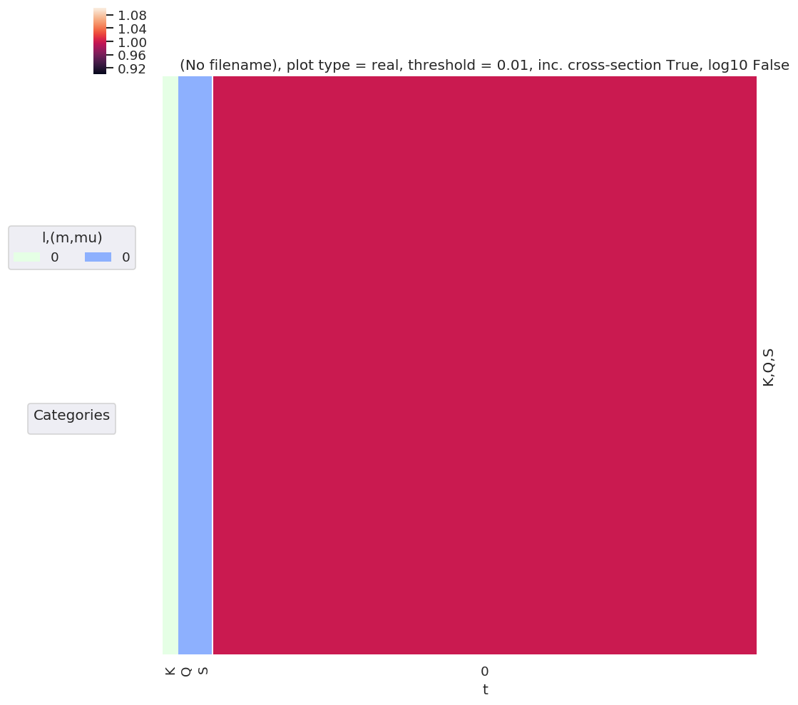
daPlot, daPlotpd, legendList, gFig = ep.lmPlot(AKQS, xDim = 't', pType = 'r', squeeze = False)  # Note squeeze = False required for 1D case (should add this to code!)
daPlotpd
Plotting data (No filename), pType=r, thres=0.01, with Seaborn
No handles with labels found to put in legend.
[5]:
| t | 0 | ||
|---|---|---|---|
| K | Q | S | |
| 0 | 0 | 0 | 1.0 |
[6]:
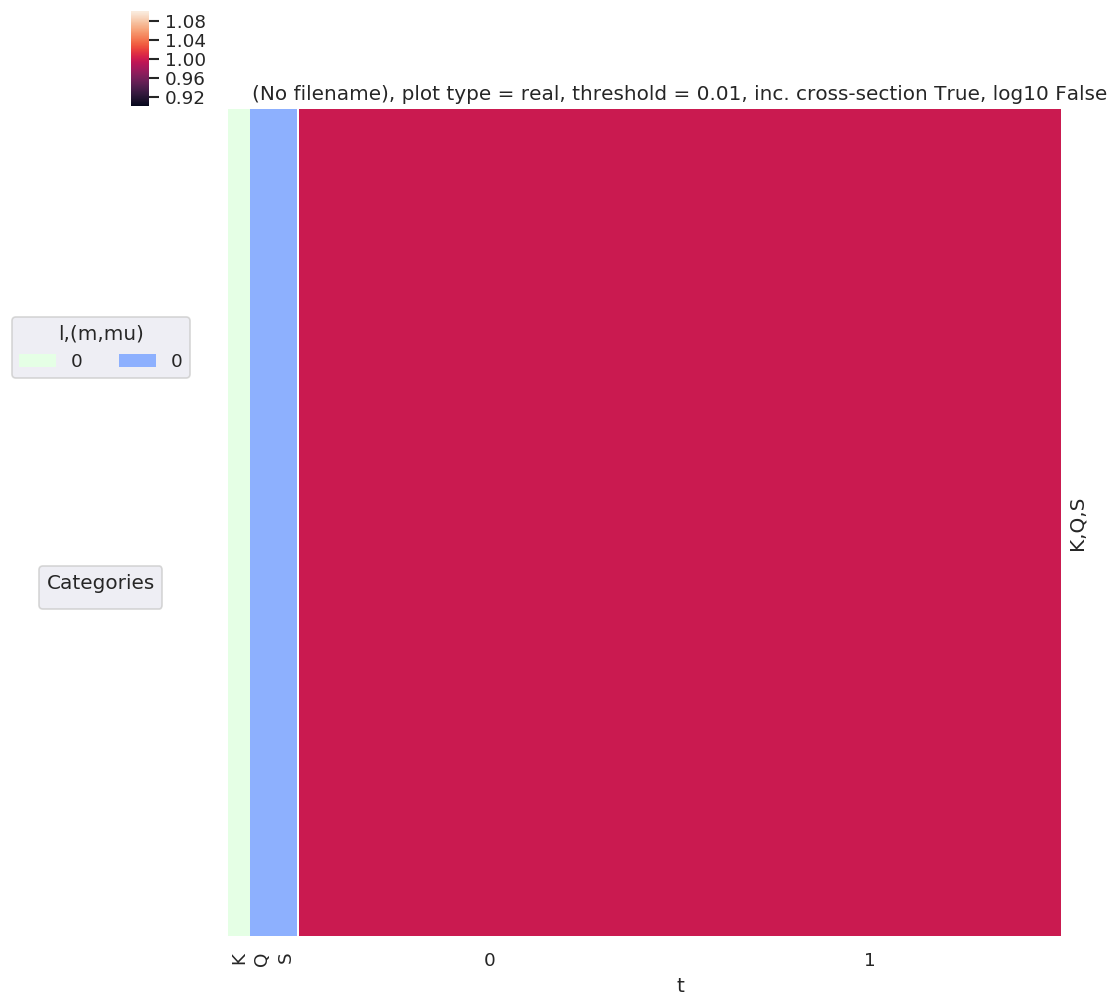
# Test multiple t points
AKQS = ep.setADMs(ADMs = [0,0,0,1,1], t=[0,1])
daPlot, daPlotpd, legendList, gFig = ep.lmPlot(AKQS, xDim = 't', pType = 'r', squeeze = False)  # Note squeeze = False required for 1D case (should add this to code!)
daPlotpd
Plotting data (No filename), pType=r, thres=0.01, with Seaborn
No handles with labels found to put in legend.
[6]:
| t | 0 | 1 | ||
|---|---|---|---|---|
| K | Q | S | ||
| 0 | 0 | 0 | 1.0 | 1.0 |
[7]:
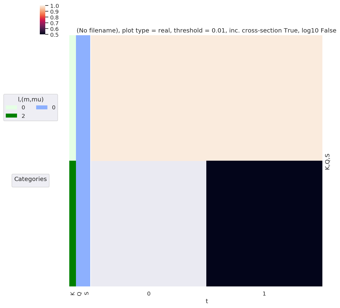
# Test additional time-dependent values
AKQS = ep.setADMs(ADMs = [[0,0,0,1,1],[2,0,0,0,0.5]], t=[0,1])    # Nested list or np.array OK.
# AKQS = ep.setADMs(ADMs = np.array([[0,0,0,1,1],[2,0,0,0,0.5]]), t=[0,1])
daPlot, daPlotpd, legendList, gFig = ep.lmPlot(AKQS, xDim = 't', pType = 'r', squeeze = False)  # Note squeeze = False required for 1D case (should add this to code!)
daPlotpd
No handles with labels found to put in legend.
Plotting data (No filename), pType=r, thres=0.01, with Seaborn
[7]:
| t | 0 | 1 | ||
|---|---|---|---|---|
| K | Q | S | ||
| 0 | 0 | 0 | 1.0 | 1.0 |
| 2 | 0 | 0 | NaN | 0.5 |
Alignment tensor
As previously defined:
Function dev
Based on existing MF functions, see ep.geomFunc.geomCalc and ep.geomFunc.mfblmGeom.
Most similar to existing betaTerm() function, which also has product of 3j terms in a similar manner.
[8]:
# Generate QNs - code adapted from ep.geomFunc.geomUtils.genllL(Lmin = 0, Lmax = 10, mFlag = True):

# Generate QNs for deltaKQS term - 3j product term
def genKQSterms(Kmin = 0, Kmax = 2, mFlag = True):
    # Set QNs for calculation, (l,m,mp)
    QNs = []
    for P in np.arange(0, 2+1):    # HARD-CODED R for testing - should get from EPR tensor defn. in full calcs.
        for K in np.arange(Kmin, Kmax+1):  # Eventually this will come from alignment term
            for L in np.arange(np.abs(P-K), P+K+1):  # Allowed L given P and K defined

                if mFlag:    # Include "m" (or equivalent) terms?
                    mMax = L
                    RMax = P
                    QMax = K
                else:
                    mMax = 0
                    RMax = 0
                    QMax = 0

                for R in np.arange(-RMax, RMax+1):
                    for Q in np.arange(-QMax, QMax+1):
                        #for M in np.arange(np.abs(l-lp), l+lp+1):
#                         for M in np.arange(-mMax, mMax+1):
                            # Set M - note this implies specific phase choice.
                            # M = -(m+mp)
                            # M = (-m+mp)
                            # if np.abs(M) <= L:  # Skip terms with invalid M
                            #     QNs.append([l, lp, L, m, mp, M])

                        # Run for all possible M
                        for M in np.arange(-L, L+1):
                            QNs.append([P, K, L, R, Q, M])

    return np.array(QNs)


# Generate QNs from EPR + AKQS tensors
def genKQStermsFromTensors(EPR, AKQS, uniqueFlag = True, phaseConvention = 'S'):
    '''
    Generate all QNs for :math:`\Delta_{L,M}(K,Q,S)` from existing tensors (Xarrays) :math:`E_{P,R}` and :math:`A^K_{Q,S}`.

    Cf. :py:func:`epsproc.geomFunc.genllpMatE`, code adapted from there.

    Parameters
    ----------
    matE : Xarray
        Xarray containing matrix elements, with QNs (l,m), as created by :py:func:`readMatEle`

    uniqueFlag : bool, default = True
        Check for duplicates and remove (can occur with some forms of matrix elements).

    mFlag : bool, optional, default = True
        m, mp take all passed values if mFlag=True, or =0 only if mFlag=False

    phaseConvention : optional, str, default = 'S'
        Set phase conventions with :py:func:`epsproc.geomCalc.setPhaseConventions`.
        To use preset phase conventions, pass existing dictionary.
        If matE.attrs['phaseCons'] is already set, this will be used instead of passed args.


    Returns
    -------
    QNs1, QNs2 : two 2D np.arrays
        Values take all allowed combinations ['P','K','L','R','Q','M'] and ['P','K','L','Rp','S','S-Rp'] from supplied matE.
        Note phase conventions not applied to QN lists as yet.

    To do
    -----
    - Implement output options (see dev. function w3jTable).

    '''

    # Local import.
    from epsproc.geomFunc.geomCalc import setPhaseConventions

    # For transparency/consistency with subfunctions, str/dict now set in setPhaseConventions()
    if 'phaseCons' in EPR.attrs.keys():
        phaseCons = EPR.attrs['phaseCons']
    else:
        phaseCons = setPhaseConventions(phaseConvention = phaseConvention)

    # Get QNs from inputs
    KQScoords = AKQS.unstack().coords  # Use unstack here, or np.unique(matE.l), to avoid duplicates
    PRcoords = EPR.unstack().coords

    # Use passed (m,mp) values, or run for m=mp=0 only.
#     if mFlag:
#         mList = matE.unstack().m.values
#     else:
#         mList = 0

    # Set QNs for calculation, one set for each 3j term
    QNs1 = []
    QNs2 = []
    for P in PRcoords['P'].values:   # Note dictionary syntax for coords objects
        for K in KQScoords['K'].values:
            for L in np.arange(np.abs(P-K), P+K+1):  # Allowed L given P and K defined

#                 if mFlag:    # Include "m" (or equivalent) terms?
#                     mMax = L
#                     RMax = P
#                     QMax = K
#                 else:
#                     mMax = 0
#                     RMax = 0
#                     QMax = 0

                for R in PRcoords['R'].values:
                    for Q in KQScoords['Q'].values:

                        # Set M, with +/- phase convention - TBC MAY BE INCORRECT IN THIS CASE/CONTEXT?
                        # Note that setting phaseCons['afblmCons']['negM']  = phaseCons['genMatEcons']['negm'] is current default case, but doesn't have to be!
                        if phaseCons['genMatEcons']['negm']:
                            M = (-R+Q)  # Case for M -> -M switch
                        else:
                            M = -(R+Q)  # Usual phase convention.

                        QNs1.append([P, K, L, R, Q, M])

                # Set Rp and S - these are essentially independent of R,Q,M, but keep nested for full dim output.
                for Rp in PRcoords['R'].values:
                    for S in KQScoords['S'].values:
                        SRp = S-Rp  # Set final 3j term, S-Rp

                        QNs2.append([P, K, L, Rp, S, SRp])

                            #for M in np.arange(np.abs(l-lp), l+lp+1):
    #                         for M in np.arange(-mMax, mMax+1):
                                # Set M - note this implies specific phase choice.
                                # M = -(m+mp)
                                # M = (-m+mp)
                                # if np.abs(M) <= L:  # Skip terms with invalid M
                                #     QNs.append([l, lp, L, m, mp, M])

                            # Run for all possible M
    #                         for M in np.arange(-L, L+1):
    #                             QNs.append([P, K, L, R, Q, M])


    if uniqueFlag:
        return np.unique(QNs1, axis = 0), np.unique(QNs2, axis = 0)
    else:
        return np.array(QNs1), np.array(QNs2)
[9]:
test = genKQSterms()
# test.tolist()   # Use tolist() to get full array output (not truncated by np)
test.shape
[9]:
(1225, 6)
[10]:
# Can also just use existing fn.
test2 = ep.geomFunc.genllL(Lmax=2)
test2.shape
[10]:
(1225, 6)
[11]:
# Also QN list fn - checks and removes duplicates
QNs = ep.geomFunc.genllL(Lmax=2)
test3 = ep.geomFunc.geomUtils.genllLList(QNs, uniqueFlag = True, mFlag = True)

test3.shape
[11]:
(1225, 6)
All QNs
[12]:
# Then calc 3js.... as per betaTerm
form = 'xdaLM'  # xds
dlist1 = ['P', 'K', 'L', 'R', 'Q', 'M']
dlist2 = ['P', 'K', 'L', 'Rp', 'S', 'S-Rp']

QNs = ep.geomFunc.genllL(Lmax=2)
[13]:
# Set phase conventions for this case, extending existing structure
phaseCons = ep.geomFunc.setPhaseConventions('E')

phaseCons['afblmCons'] = {}

# (+/-)M phase selection, set as per existing code, betaCons['negM'] = genMatEcons['negm']       # Use -M term in 3j? Should be anti-correlated with genMatEcons['negm']...? 31/03/20 NOW correlated with mfblmCons['Mphase']
# Note this is correlated with QN generation in genllpMatE() - should set equivalent fn for alignment terms.
# In existing case this arises from M = (-m+mp) or M = -(m+mp) choice.
phaseCons['afblmCons']['negM'] = phaseCons['genMatEcons']['negm']
phaseCons['afblmCons']['negQ'] = True
phaseCons['afblmCons']['negS'] = True


# Apply phase conventions to input QNs
#         if phaseCons['mfblmCons']['BLMmPhase']:
#             QNsBLMtable[:,3] *= -1
#             QNsBLMtable[:,5] *= -1
[14]:
# Calculate two 3j terms, with respective QN sets
thrj1 = ep.geomFunc.w3jTable(QNs = QNs, nonzeroFlag = True, form = form, dlist = dlist1)
thrj2 = ep.geomFunc.w3jTable(QNs = QNs, nonzeroFlag = True, form = form, dlist = dlist2)
[15]:
# Multiplication term...

testMult = thrj1.unstack() * thrj2.unstack()

# This can get large quickly - for Kmax=2 already have 2e6 terms
[16]:
# plotDimsRed = ['l', 'm', 'lp', 'mp']
xDim = {'LM':['L','M']}
# daPlot, daPlotpd, legendList, gFig = ep.lmPlot(testMult, plotDims=plotDimsRed, xDim=xDim, pType = 'r')
daPlot, daPlotpd, legendList, gFig = ep.lmPlot(testMult, xDim=xDim, pType = 'r')
Set dataType (No dataType)
Plotting data (No filename), pType=r, thres=0.01, with Seaborn
C:\Users\femtolab\.conda\envs\ePSdev\lib\site-packages\xarray\core\nputils.py:215: RuntimeWarning:

All-NaN slice encountered
Reduced QNs set
[17]:
# Then calc 3js.... as per betaTerm
form = 'xdaLM'  # xds
dlist1 = ['P', 'K', 'L', 'R', 'Q', 'M']
dlist2 = ['P', 'K', 'L', 'Rp', 'S', 'S-Rp']

# Calculate two 3j terms, with respective QN sets
thrj1 = ep.geomFunc.w3jTable(QNs = QNs, nonzeroFlag = True, form = form, dlist = dlist1)
thrj2 = ep.geomFunc.w3jTable(QNs = QNs, nonzeroFlag = True, form = form, dlist = dlist2)
[18]:
# With subselection (currently don't have QN generation fnc of correct form - see geomUtils)
# from epsproc.util import matEleSelector
# thrj1Sel = ep.util.matEleSelector(thrj1, inds = {'Q':0}, sq=False)
[19]:
# Check 3j terms
xDim = {'LM':['L','M']}
daPlot, daPlotpd, legendList, gFig = ep.lmPlot(thrj1, xDim=xDim, pType = 'r')

xDim = {'LM':['L','S-Rp']}
daPlot, daPlotpd, legendList, gFig = ep.lmPlot(thrj2.sel({'S':0}), xDim=xDim, pType = 'r')
C:\Users\femtolab\.conda\envs\ePSdev\lib\site-packages\xarray\core\nputils.py:215: RuntimeWarning:

All-NaN slice encountered
Plotting data (No filename), pType=r, thres=0.01, with Seaborn
C:\Users\femtolab\.conda\envs\ePSdev\lib\site-packages\xarray\core\nputils.py:215: RuntimeWarning:

All-NaN slice encountered
Plotting data (No filename), pType=r, thres=0.01, with Seaborn
[20]:
# Multiplication term...

testMultSub = thrj1.unstack().sel({'Q':0}) * thrj2.unstack().sel({'S':0})   # SLOW, 91125 elements. ACTUALLY - much faster after a reboot. Sigh.

testMultSub2 = thrj1.sel({'Q':0}).unstack() * thrj2.sel({'S':0}).unstack()  # FAST, 28125 elements. Possible issue with which dims are dropped - check previous notes!

# This can get large quickly - for Kmax=2 already have 2e6 terms

testMultSub.notnull().sum() # == 194 for Kmax = 2, Q=S=0
testMultSub2.notnull().sum() # == 194 for Kmax = 2, Q=S=0  OK
[20]:
<xarray.DataArray 'w3jStacked' ()>
array(194)
Coordinates:
    Q        int64 0
    S        int64 0
[20]:
<xarray.DataArray 'w3jStacked' ()>
array(194)
[21]:
# plotDimsRed = ['l', 'm', 'lp', 'mp']
xDim = {'LM':['L','M']}
# daPlot, daPlotpd, legendList, gFig = ep.lmPlot(testMult, plotDims=plotDimsRed, xDim=xDim, pType = 'r')
daPlot, daPlotpd, legendList, gFig = ep.lmPlot(testMultSub, xDim=xDim, pType = 'r')
Set dataType (No dataType)
Plotting data (No filename), pType=r, thres=0.01, with Seaborn
C:\Users\femtolab\.conda\envs\ePSdev\lib\site-packages\xarray\core\nputils.py:215: RuntimeWarning:

All-NaN slice encountered
[22]:
# plotDimsRed = ['l', 'm', 'lp', 'mp']
xDim = {'LM':['L','M']}
# daPlot, daPlotpd, legendList, gFig = ep.lmPlot(testMult, plotDims=plotDimsRed, xDim=xDim, pType = 'r')
daPlot, daPlotpd, legendList, gFig = ep.lmPlot(testMultSub2, xDim=xDim, pType = 'r')
Set dataType (No dataType)
Plotting data (No filename), pType=r, thres=0.01, with Seaborn
C:\Users\femtolab\.conda\envs\ePSdev\lib\site-packages\xarray\core\nputils.py:215: RuntimeWarning:

All-NaN slice encountered
Plots appear to be the same, aside from ordering of M terms(?)
QNs from existing tensors
[23]:
phaseConvention = 'E'

# Set polarisation term
p=[0]
EPRX = geomCalc.EPR(form = 'xarray', p = p, nonzeroFlag = True, phaseConvention = phaseConvention).unstack().sel({'R-p':0}).drop('R-p') # Set for R-p = 0 for p=0 case (redundant coord) - need to fix in e-field mult term!
EPRXresort = EPRX.squeeze(['l','lp']).drop(['l','lp'])  # Safe squeeze & drop of selected singleton dims only.

# Set alignment terms (inc. time-dependence)
AKQS = ep.setADMs(ADMs = [[0,0,0,1,1],[2,0,0,0,0.5]], t=[0,1])    # Nested list or np.array OK.
[24]:
# Calculate alignment term - this cell should form core function, cf. betaTerm() etc.

# Set QNs
QNs1, QNs2 = genKQStermsFromTensors(EPRXresort, AKQS, uniqueFlag = True, phaseConvention = phaseConvention)

# Then calc 3js.... as per betaTerm
form = 'xdaLM'  # xds
dlist1 = ['P', 'K', 'L', 'R', 'Q', 'M']
dlist2 = ['P', 'K', 'L', 'Rp', 'S', 'S-Rp']

# Copy QNs and apply any additional phase conventions
QNs1DeltaTable = QNs1.copy()
QNs2DeltaTable = QNs2.copy()

# Set additional phase cons here - these will be set in master function eventually!
# NOTE - only testing for Q=S=0 case initially.
phaseCons['afblmCons']['negM'] = phaseCons['genMatEcons']['negm']  # IF SET TO TRUE THIS KNOCKS OUT M!=0 terms - not sure if this is correct here, depends also on phase cons in genKQStermsFromTensors().
                                                                    # Yeah, looks like phase error in current case, get terms with R=M, instead of R=-M
                                                                    # Confusion is due to explicit assignment of +/-M terms in QN generation (only allowed terms), which *already* enforces this phase convention.
phaseCons['afblmCons']['negQ'] = True
phaseCons['afblmCons']['negS'] = True

# Switch signs (m,M) before 3j calcs.
if phaseCons['afblmCons']['negQ']:
    QNs1DeltaTable[:,4] *= -1

# Switch sign Q > -Q before 3j calcs.
if phaseCons['afblmCons']['negM']:
    QNs1DeltaTable[:,5] *= -1

# Switch sign S > -S before 3j calcs.
if phaseCons['afblmCons']['negS']:
    QNs2DeltaTable[:,4] *= -1


# Calculate two 3j terms, with respective QN sets
thrj1 = ep.geomFunc.w3jTable(QNs = QNs1DeltaTable, nonzeroFlag = True, form = form, dlist = dlist1)
thrj2 = ep.geomFunc.w3jTable(QNs = QNs2DeltaTable, nonzeroFlag = True, form = form, dlist = dlist2)

# Multiply
thrjMult = thrj1.unstack() * thrj2.unstack()

# Additional terms & multiplications
Kdegen = np.sqrt(2*thrjMult.K + 1)
KQphase = np.power(-1, np.abs(thrjMult.K + thrjMult.Q))

DeltaKQS =  Kdegen * KQphase * thrjMult

# AF term
AFterm = (DeltaKQS * AKQS.unstack()).sum({'K','Q','S'})
[25]:
thrjMult.notnull().sum() # == 69 for test case with all phase switches on, and same for no phase switches (in test case Q=S=0 in any case!)
[25]:
<xarray.DataArray 'w3jStacked' ()>
array(69)
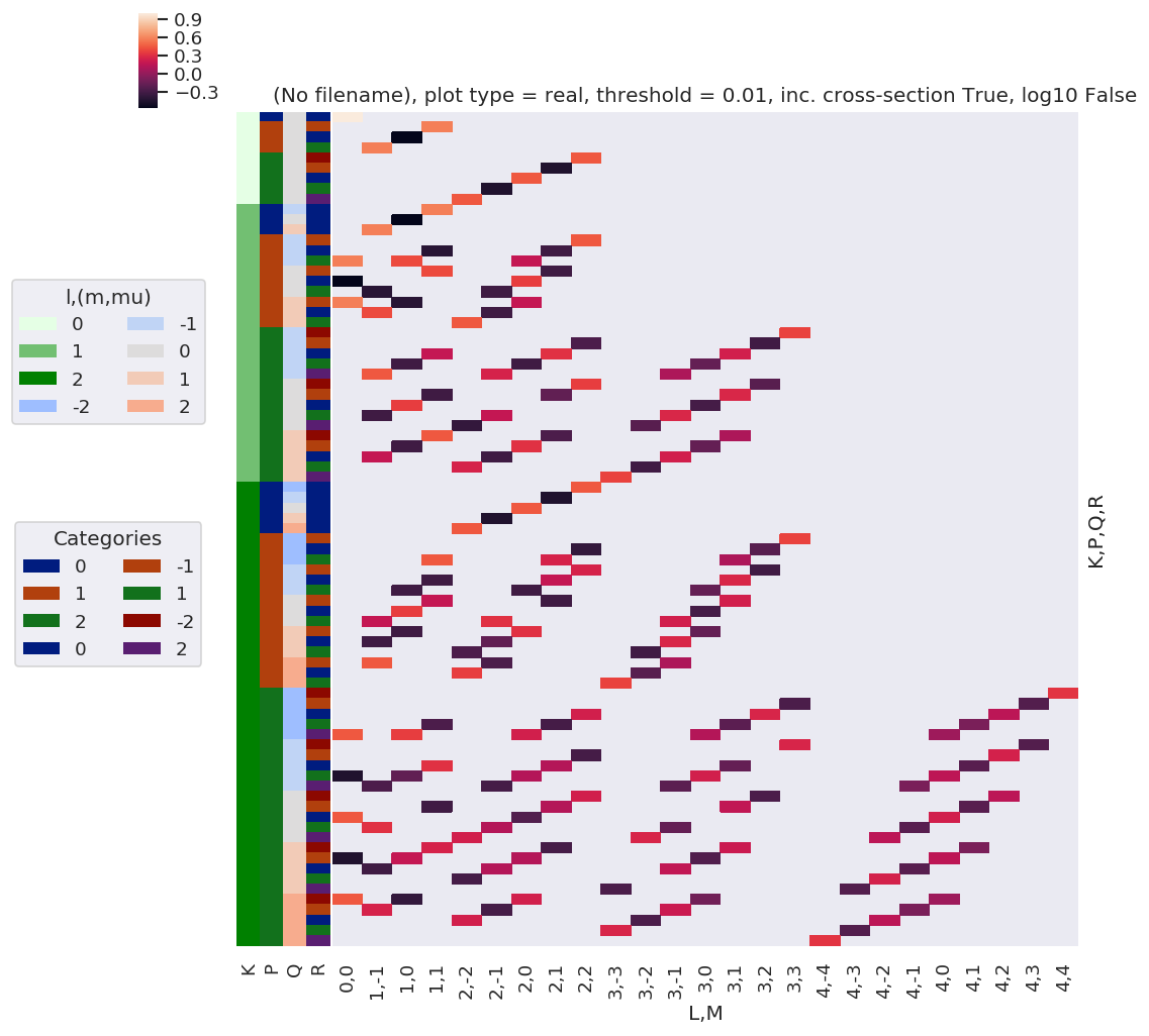
[26]:
# Plot
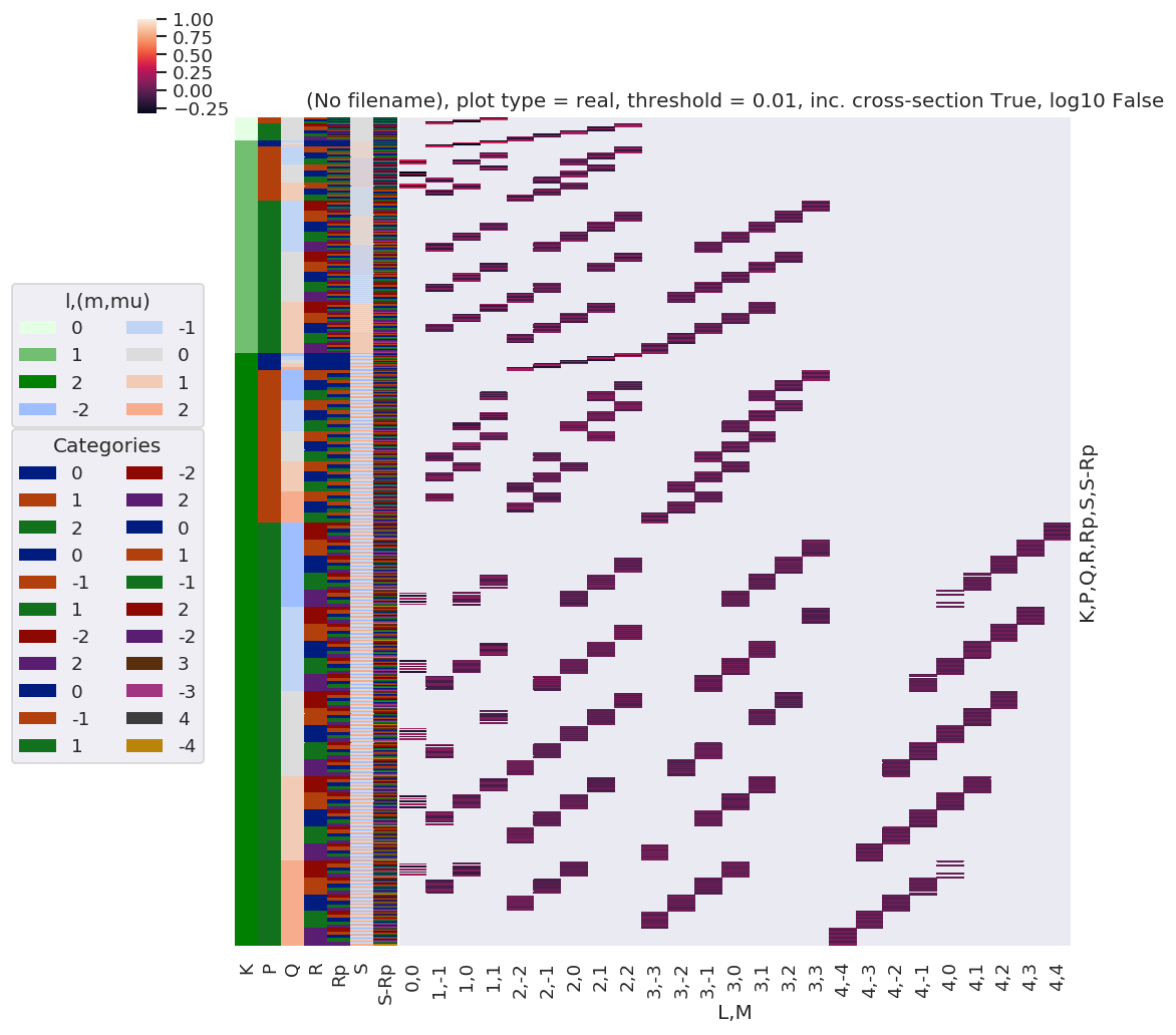
xDim = {'LM':['L','M']}
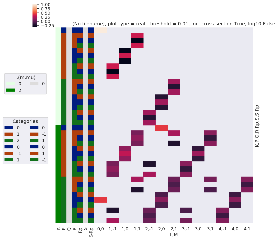
# daPlot, daPlotpd, legendList, gFig = ep.lmPlot(testMult, plotDims=plotDimsRed, xDim=xDim, pType = 'r')
daPlot, daPlotpd, legendList, gFig = ep.lmPlot(DeltaKQS, xDim=xDim, pType = 'r')
Set dataType (No dataType)
Plotting data (No filename), pType=r, thres=0.01, with Seaborn
C:\Users\femtolab\.conda\envs\ePSdev\lib\site-packages\xarray\core\nputils.py:215: RuntimeWarning:

All-NaN slice encountered
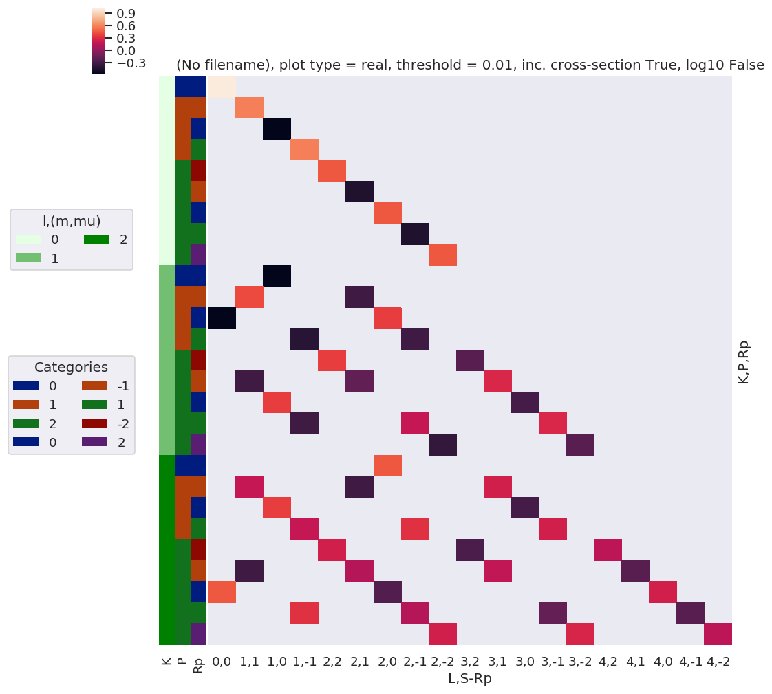
[27]:
# Plot
xDim = {'LM':['L','M']}
# daPlot, daPlotpd, legendList, gFig = ep.lmPlot(testMult, plotDims=plotDimsRed, xDim=xDim, pType = 'r')
daPlot, daPlotpd, legendList, gFig = ep.lmPlot(AFterm, xDim=xDim, pType = 'r')
daPlotpd
Set dataType (No dataType)
Plotting data (No filename), pType=r, thres=0.01, with Seaborn
No handles with labels found to put in legend.
[27]:
| L | 0 | 1 | 2 | 3 | 4 | ||||||||||||
|---|---|---|---|---|---|---|---|---|---|---|---|---|---|---|---|---|---|
| M | 0 | -1 | 0 | 1 | -1 | 0 | 1 | -1 | 0 | 1 | -1 | 0 | 1 | ||||
| P | R | Rp | S-Rp | t | |||||||||||||
| 0 | 0 | 0 | 0 | 0 | 1.000000 | NaN | NaN | NaN | NaN | NaN | NaN | NaN | NaN | NaN | NaN | NaN | NaN |
| 1 | 1.000000 | NaN | NaN | NaN | NaN | 0.223607 | NaN | NaN | NaN | NaN | NaN | NaN | NaN | ||||
| 1 | -1 | -1 | 1 | 0 | NaN | NaN | NaN | 0.333333 | NaN | NaN | NaN | NaN | NaN | NaN | NaN | NaN | NaN |
| 1 | NaN | NaN | NaN | 0.370601 | NaN | NaN | 0.111803 | NaN | NaN | 0.063888 | NaN | NaN | NaN | ||||
| 0 | 0 | 0 | NaN | NaN | NaN | -0.333333 | NaN | NaN | NaN | NaN | NaN | NaN | NaN | NaN | NaN | ||
| 1 | NaN | NaN | NaN | -0.258798 | NaN | NaN | NaN | NaN | NaN | -0.078246 | NaN | NaN | NaN | ||||
| 1 | -1 | 0 | NaN | NaN | NaN | 0.333333 | NaN | NaN | NaN | NaN | NaN | NaN | NaN | NaN | NaN | ||
| 1 | NaN | NaN | NaN | 0.370601 | NaN | NaN | -0.111803 | NaN | NaN | 0.063888 | NaN | NaN | NaN | ||||
| 0 | -1 | 1 | 0 | NaN | NaN | -0.333333 | NaN | NaN | NaN | NaN | NaN | NaN | NaN | NaN | NaN | NaN | |
| 1 | NaN | NaN | -0.258798 | NaN | NaN | NaN | NaN | NaN | -0.078246 | NaN | NaN | NaN | NaN | ||||
| 0 | 0 | 0 | NaN | NaN | 0.333333 | NaN | NaN | NaN | NaN | NaN | NaN | NaN | NaN | NaN | NaN | ||
| 1 | NaN | NaN | 0.482405 | NaN | NaN | NaN | NaN | NaN | 0.095831 | NaN | NaN | NaN | NaN | ||||
| 1 | -1 | 0 | NaN | NaN | -0.333333 | NaN | NaN | NaN | NaN | NaN | NaN | NaN | NaN | NaN | NaN | ||
| 1 | NaN | NaN | -0.258798 | NaN | NaN | NaN | NaN | NaN | -0.078246 | NaN | NaN | NaN | NaN | ||||
| 1 | -1 | 1 | 0 | NaN | 0.333333 | NaN | NaN | NaN | NaN | NaN | NaN | NaN | NaN | NaN | NaN | NaN | |
| 1 | NaN | 0.370601 | NaN | NaN | -0.111803 | NaN | NaN | 0.063888 | NaN | NaN | NaN | NaN | NaN | ||||
| 0 | 0 | 0 | NaN | -0.333333 | NaN | NaN | NaN | NaN | NaN | NaN | NaN | NaN | NaN | NaN | NaN | ||
| 1 | NaN | -0.258798 | NaN | NaN | NaN | NaN | NaN | -0.078246 | NaN | NaN | NaN | NaN | NaN | ||||
| 1 | -1 | 0 | NaN | 0.333333 | NaN | NaN | NaN | NaN | NaN | NaN | NaN | NaN | NaN | NaN | NaN | ||
| 1 | NaN | 0.370601 | NaN | NaN | 0.111803 | NaN | NaN | 0.063888 | NaN | NaN | NaN | NaN | NaN | ||||
| 2 | -1 | -1 | 1 | 0 | NaN | NaN | NaN | NaN | NaN | NaN | 0.200000 | NaN | NaN | NaN | NaN | NaN | NaN |
| 1 | NaN | NaN | NaN | 0.111803 | NaN | NaN | 0.215972 | NaN | NaN | 0.031944 | NaN | NaN | 0.053240 | ||||
| 0 | 0 | 0 | NaN | NaN | NaN | NaN | NaN | NaN | -0.200000 | NaN | NaN | NaN | NaN | NaN | NaN | ||
| 1 | NaN | NaN | NaN | NaN | NaN | NaN | -0.231944 | NaN | NaN | NaN | NaN | NaN | -0.058321 | ||||
| 1 | -1 | 0 | NaN | NaN | NaN | NaN | NaN | NaN | 0.200000 | NaN | NaN | NaN | NaN | NaN | NaN | ||
| 1 | NaN | NaN | NaN | -0.111803 | NaN | NaN | 0.215972 | NaN | NaN | -0.031944 | NaN | NaN | 0.053240 | ||||
| 0 | -1 | 1 | 0 | NaN | NaN | NaN | NaN | NaN | -0.200000 | NaN | NaN | NaN | NaN | NaN | NaN | NaN | |
| 1 | NaN | NaN | NaN | NaN | NaN | -0.231944 | NaN | NaN | NaN | NaN | NaN | -0.058321 | NaN | ||||
| 0 | 0 | 0 | NaN | NaN | NaN | NaN | NaN | 0.200000 | NaN | NaN | NaN | NaN | NaN | NaN | NaN | ||
| 1 | 0.223607 | NaN | NaN | NaN | NaN | 0.263888 | NaN | NaN | NaN | NaN | NaN | 0.063888 | NaN | ||||
| 1 | -1 | 0 | NaN | NaN | NaN | NaN | NaN | -0.200000 | NaN | NaN | NaN | NaN | NaN | NaN | NaN | ||
| 1 | NaN | NaN | NaN | NaN | NaN | -0.231944 | NaN | NaN | NaN | NaN | NaN | -0.058321 | NaN | ||||
| 1 | -1 | 1 | 0 | NaN | NaN | NaN | NaN | 0.200000 | NaN | NaN | NaN | NaN | NaN | NaN | NaN | NaN | |
| 1 | NaN | -0.111803 | NaN | NaN | 0.215972 | NaN | NaN | -0.031944 | NaN | NaN | 0.053240 | NaN | NaN | ||||
| 0 | 0 | 0 | NaN | NaN | NaN | NaN | -0.200000 | NaN | NaN | NaN | NaN | NaN | NaN | NaN | NaN | ||
| 1 | NaN | NaN | NaN | NaN | -0.231944 | NaN | NaN | NaN | NaN | NaN | -0.058321 | NaN | NaN | ||||
| 1 | -1 | 0 | NaN | NaN | NaN | NaN | 0.200000 | NaN | NaN | NaN | NaN | NaN | NaN | NaN | NaN | ||
| 1 | NaN | 0.111803 | NaN | NaN | 0.215972 | NaN | NaN | 0.031944 | NaN | NaN | 0.053240 | NaN | NaN | ||||
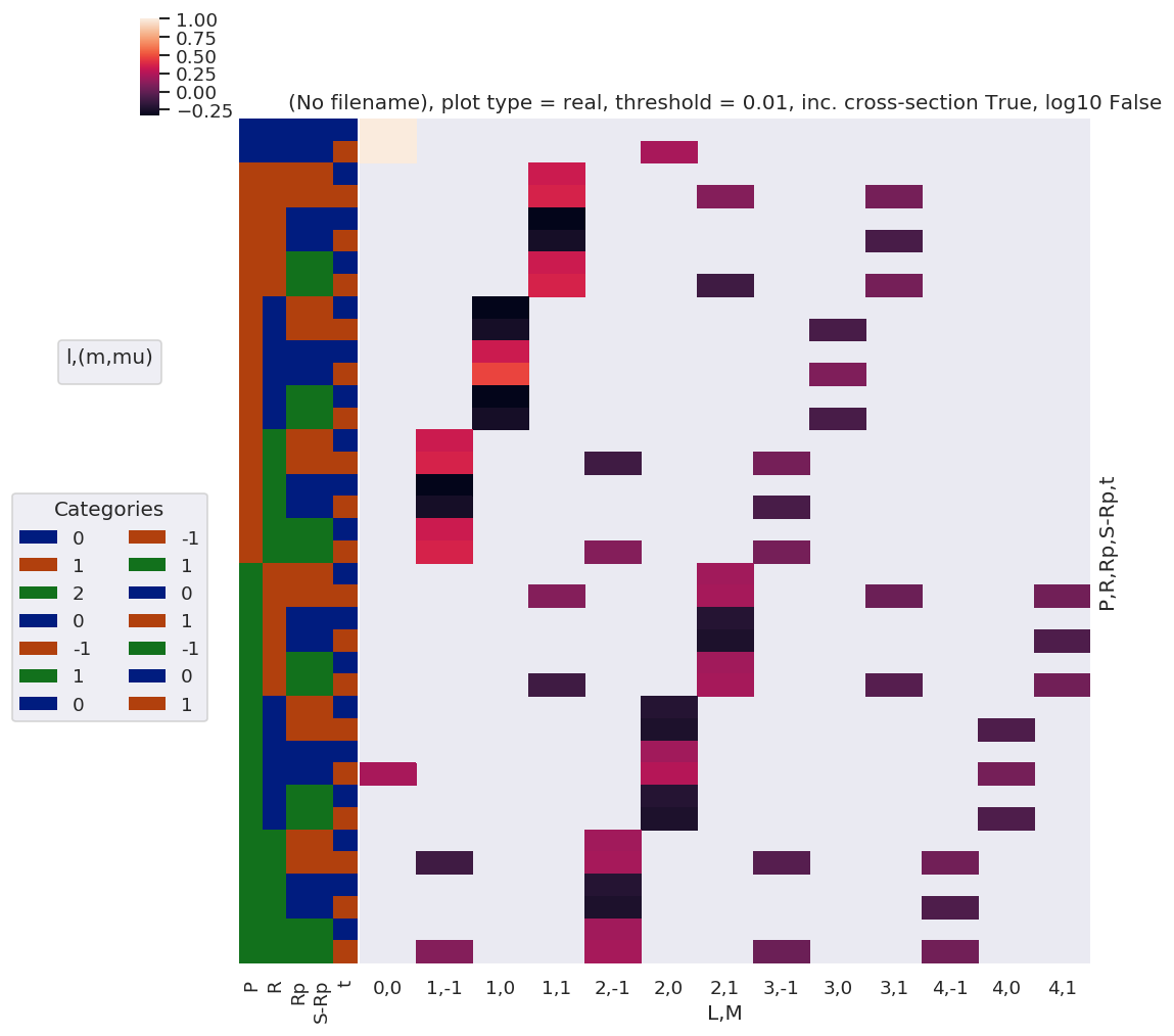
Note here that there are blocks of non-zero terms with M=+/-1, these should drop out later (?) by sums over symmetry and/or other 3j terms… TBC…
Lambda term redux
Use existing function and force/sub-select terms…
[28]:
# Code adapted from mfblmXprod()

eulerAngs = np.array([0,0,0], ndmin=2)
# RX = ep.setPolGeoms(eulerAngs = eulerAngs)   # This throws error in geomCalc.MFproj???? Something to do with form of terms passed to wD, line 970 vs. 976 in geomCalc.py
RX = ep.setPolGeoms()   # (0,0,0) term in geomCalc.MFproj OK.

lambdaTerm, lambdaTable, lambdaD, QNsLambda = geomCalc.MFproj(RX = RX, form = 'xarray', phaseConvention = phaseConvention)
# lambdaTermResort = lambdaTerm.squeeze().drop('l').drop('lp')   # This removes photon (l,lp) dims fully.
lambdaTermResort = lambdaTerm.squeeze(['l','lp']).drop(['l','lp']).sel({'Labels':'z'})  # Safe squeeze & drop of selected singleton dims only.
[29]:
# Plot
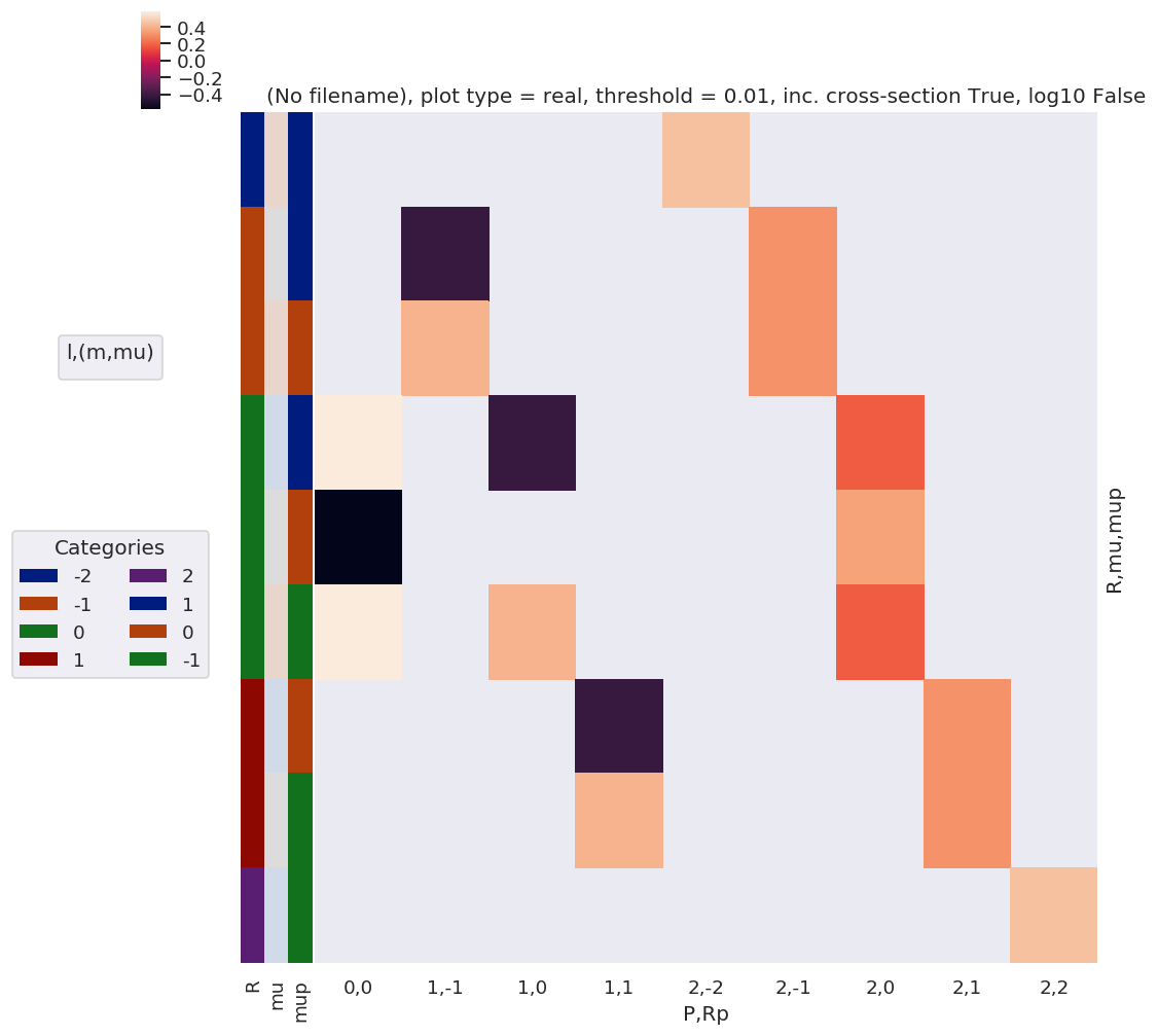
xDim = {'PRp':['P','Rp']}
# daPlot, daPlotpd, legendList, gFig = ep.lmPlot(testMult, plotDims=plotDimsRed, xDim=xDim, pType = 'r')
daPlot, daPlotpd, legendList, gFig = ep.lmPlot(lambdaTermResort, xDim=xDim, pType = 'r')
daPlotpd
Plotting data (No filename), pType=r, thres=0.01, with Seaborn
No handles with labels found to put in legend.
[29]:
| P | 0 | 1 | 2 | ||||||||
|---|---|---|---|---|---|---|---|---|---|---|---|
| Rp | 0 | -1 | 0 | 1 | -2 | -1 | 0 | 1 | 2 | ||
| R | mu | mup | |||||||||
| -2 | 1 | 1 | NaN | NaN | NaN | NaN | 0.447214 | NaN | NaN | NaN | NaN |
| -1 | 0 | 1 | NaN | -0.408248 | NaN | NaN | NaN | 0.316228 | NaN | NaN | NaN |
| 1 | 0 | NaN | 0.408248 | NaN | NaN | NaN | 0.316228 | NaN | NaN | NaN | |
| 0 | -1 | 1 | 0.57735 | NaN | -0.408248 | NaN | NaN | NaN | 0.182574 | NaN | NaN |
| 0 | 0 | -0.57735 | NaN | NaN | NaN | NaN | NaN | 0.365148 | NaN | NaN | |
| 1 | -1 | 0.57735 | NaN | 0.408248 | NaN | NaN | NaN | 0.182574 | NaN | NaN | |
| 1 | -1 | 0 | NaN | NaN | NaN | -0.408248 | NaN | NaN | NaN | 0.316228 | NaN |
| 0 | -1 | NaN | NaN | NaN | 0.408248 | NaN | NaN | NaN | 0.316228 | NaN | |
| 2 | -1 | -1 | NaN | NaN | NaN | NaN | NaN | NaN | NaN | NaN | 0.447214 |
Check component terms are as expected
Should have R = Rp for z case, and wD terms = 1 or 0.
[30]:
lambdaTablepd, _ = ep.util.multiDimXrToPD(lambdaTable, colDims=xDim, dropna=True)
lambdaTablepd
[30]:
| P | 0 | 1 | 2 | ||||||||||
|---|---|---|---|---|---|---|---|---|---|---|---|---|---|
| Rp | 0 | -1 | 0 | 1 | -2 | -1 | 0 | 1 | 2 | ||||
| R | l | lp | mu | mup | |||||||||
| -2 | 1 | 1 | -1 | -1 | NaN | NaN | NaN | NaN | NaN | NaN | NaN | NaN | 0.447214 |
| 0 | NaN | NaN | NaN | NaN | NaN | NaN | NaN | -0.316228 | NaN | ||||
| 1 | NaN | NaN | NaN | NaN | NaN | NaN | 0.182574 | NaN | NaN | ||||
| 0 | -1 | NaN | NaN | NaN | NaN | NaN | NaN | NaN | -0.316228 | NaN | |||
| 0 | NaN | NaN | NaN | NaN | NaN | NaN | 0.365148 | NaN | NaN | ||||
| 1 | NaN | NaN | NaN | NaN | NaN | -0.316228 | NaN | NaN | NaN | ||||
| 1 | -1 | NaN | NaN | NaN | NaN | NaN | NaN | 0.182574 | NaN | NaN | |||
| 0 | NaN | NaN | NaN | NaN | NaN | -0.316228 | NaN | NaN | NaN | ||||
| 1 | NaN | NaN | NaN | NaN | 0.447214 | NaN | NaN | NaN | NaN | ||||
| -1 | 1 | 1 | -1 | -1 | NaN | NaN | NaN | NaN | NaN | NaN | NaN | NaN | 0.447214 |
| 0 | NaN | NaN | NaN | 0.408248 | NaN | NaN | NaN | -0.316228 | NaN | ||||
| 1 | NaN | NaN | -0.408248 | NaN | NaN | NaN | 0.182574 | NaN | NaN | ||||
| 0 | -1 | NaN | NaN | NaN | -0.408248 | NaN | NaN | NaN | -0.316228 | NaN | |||
| 0 | NaN | NaN | NaN | NaN | NaN | NaN | 0.365148 | NaN | NaN | ||||
| 1 | NaN | 0.408248 | NaN | NaN | NaN | -0.316228 | NaN | NaN | NaN | ||||
| 1 | -1 | NaN | NaN | 0.408248 | NaN | NaN | NaN | 0.182574 | NaN | NaN | |||
| 0 | NaN | -0.408248 | NaN | NaN | NaN | -0.316228 | NaN | NaN | NaN | ||||
| 1 | NaN | NaN | NaN | NaN | 0.447214 | NaN | NaN | NaN | NaN | ||||
| 0 | 1 | 1 | -1 | -1 | NaN | NaN | NaN | NaN | NaN | NaN | NaN | NaN | 0.447214 |
| 0 | NaN | NaN | NaN | 0.408248 | NaN | NaN | NaN | -0.316228 | NaN | ||||
| 1 | 0.57735 | NaN | -0.408248 | NaN | NaN | NaN | 0.182574 | NaN | NaN | ||||
| 0 | -1 | NaN | NaN | NaN | -0.408248 | NaN | NaN | NaN | -0.316228 | NaN | |||
| 0 | -0.57735 | NaN | NaN | NaN | NaN | NaN | 0.365148 | NaN | NaN | ||||
| 1 | NaN | 0.408248 | NaN | NaN | NaN | -0.316228 | NaN | NaN | NaN | ||||
| 1 | -1 | 0.57735 | NaN | 0.408248 | NaN | NaN | NaN | 0.182574 | NaN | NaN | |||
| 0 | NaN | -0.408248 | NaN | NaN | NaN | -0.316228 | NaN | NaN | NaN | ||||
| 1 | NaN | NaN | NaN | NaN | 0.447214 | NaN | NaN | NaN | NaN | ||||
| 1 | 1 | 1 | -1 | -1 | NaN | NaN | NaN | NaN | NaN | NaN | NaN | NaN | 0.447214 |
| 0 | NaN | NaN | NaN | 0.408248 | NaN | NaN | NaN | -0.316228 | NaN | ||||
| 1 | NaN | NaN | -0.408248 | NaN | NaN | NaN | 0.182574 | NaN | NaN | ||||
| 0 | -1 | NaN | NaN | NaN | -0.408248 | NaN | NaN | NaN | -0.316228 | NaN | |||
| 0 | NaN | NaN | NaN | NaN | NaN | NaN | 0.365148 | NaN | NaN | ||||
| 1 | NaN | 0.408248 | NaN | NaN | NaN | -0.316228 | NaN | NaN | NaN | ||||
| 1 | -1 | NaN | NaN | 0.408248 | NaN | NaN | NaN | 0.182574 | NaN | NaN | |||
| 0 | NaN | -0.408248 | NaN | NaN | NaN | -0.316228 | NaN | NaN | NaN | ||||
| 1 | NaN | NaN | NaN | NaN | 0.447214 | NaN | NaN | NaN | NaN | ||||
| 2 | 1 | 1 | -1 | -1 | NaN | NaN | NaN | NaN | NaN | NaN | NaN | NaN | 0.447214 |
| 0 | NaN | NaN | NaN | NaN | NaN | NaN | NaN | -0.316228 | NaN | ||||
| 1 | NaN | NaN | NaN | NaN | NaN | NaN | 0.182574 | NaN | NaN | ||||
| 0 | -1 | NaN | NaN | NaN | NaN | NaN | NaN | NaN | -0.316228 | NaN | |||
| 0 | NaN | NaN | NaN | NaN | NaN | NaN | 0.365148 | NaN | NaN | ||||
| 1 | NaN | NaN | NaN | NaN | NaN | -0.316228 | NaN | NaN | NaN | ||||
| 1 | -1 | NaN | NaN | NaN | NaN | NaN | NaN | 0.182574 | NaN | NaN | |||
| 0 | NaN | NaN | NaN | NaN | NaN | -0.316228 | NaN | NaN | NaN | ||||
| 1 | NaN | NaN | NaN | NaN | 0.447214 | NaN | NaN | NaN | NaN | ||||
[31]:
lambdaTermResortpd, _ = ep.util.multiDimXrToPD(lambdaTermResort, colDims=xDim, dropna=True)
lambdaTermResortpd

# Think this is as per lambdaTable terms, just different ordering - because lambdaTable doesn't include some phase switches?
[31]:
| P | 0 | 1 | 2 | ||||||||
|---|---|---|---|---|---|---|---|---|---|---|---|
| Rp | 0 | -1 | 0 | 1 | -2 | -1 | 0 | 1 | 2 | ||
| R | mu | mup | |||||||||
| -2 | -1 | -1 | NaN | NaN | NaN | NaN | NaN | NaN | NaN | NaN | 0.000000+0.000000j |
| 0 | NaN | NaN | NaN | NaN | NaN | NaN | NaN | 0.000000+0.000000j | NaN | ||
| 1 | NaN | NaN | NaN | NaN | NaN | NaN | 0.000000+0.000000j | NaN | NaN | ||
| 0 | -1 | NaN | NaN | NaN | NaN | NaN | NaN | NaN | 0.000000+0.000000j | NaN | |
| 0 | NaN | NaN | NaN | NaN | NaN | NaN | 0.000000+0.000000j | NaN | NaN | ||
| 1 | NaN | NaN | NaN | NaN | NaN | 0.000000+0.000000j | NaN | NaN | NaN | ||
| 1 | -1 | NaN | NaN | NaN | NaN | NaN | NaN | 0.000000+0.000000j | NaN | NaN | |
| 0 | NaN | NaN | NaN | NaN | NaN | 0.000000+0.000000j | NaN | NaN | NaN | ||
| 1 | NaN | NaN | NaN | NaN | 0.447214+0.000000j | NaN | NaN | NaN | NaN | ||
| -1 | -1 | -1 | NaN | NaN | NaN | NaN | NaN | NaN | NaN | NaN | 0.000000+0.000000j |
| 0 | NaN | NaN | NaN | 0.000000+0.000000j | NaN | NaN | NaN | 0.000000+0.000000j | NaN | ||
| 1 | NaN | NaN | 0.000000+0.000000j | NaN | NaN | NaN | 0.000000+0.000000j | NaN | NaN | ||
| 0 | -1 | NaN | NaN | NaN | 0.000000+0.000000j | NaN | NaN | NaN | 0.000000+0.000000j | NaN | |
| 0 | NaN | NaN | NaN | NaN | NaN | NaN | 0.000000+0.000000j | NaN | NaN | ||
| 1 | NaN | -0.408248+0.000000j | NaN | NaN | NaN | 0.316228+0.000000j | NaN | NaN | NaN | ||
| 1 | -1 | NaN | NaN | 0.000000+0.000000j | NaN | NaN | NaN | 0.000000+0.000000j | NaN | NaN | |
| 0 | NaN | 0.408248+0.000000j | NaN | NaN | NaN | 0.316228+0.000000j | NaN | NaN | NaN | ||
| 1 | NaN | NaN | NaN | NaN | 0.000000+0.000000j | NaN | NaN | NaN | NaN | ||
| 0 | -1 | -1 | NaN | NaN | NaN | NaN | NaN | NaN | NaN | NaN | 0.000000+0.000000j |
| 0 | NaN | NaN | NaN | 0.000000+0.000000j | NaN | NaN | NaN | 0.000000+0.000000j | NaN | ||
| 1 | 0.577350+0.000000j | NaN | -0.408248+0.000000j | NaN | NaN | NaN | 0.182574+0.000000j | NaN | NaN | ||
| 0 | -1 | NaN | NaN | NaN | 0.000000+0.000000j | NaN | NaN | NaN | 0.000000+0.000000j | NaN | |
| 0 | -0.577350+0.000000j | NaN | NaN | NaN | NaN | NaN | 0.365148+0.000000j | NaN | NaN | ||
| 1 | NaN | 0.000000+0.000000j | NaN | NaN | NaN | 0.000000+0.000000j | NaN | NaN | NaN | ||
| 1 | -1 | 0.577350+0.000000j | NaN | 0.408248+0.000000j | NaN | NaN | NaN | 0.182574+0.000000j | NaN | NaN | |
| 0 | NaN | 0.000000+0.000000j | NaN | NaN | NaN | 0.000000+0.000000j | NaN | NaN | NaN | ||
| 1 | NaN | NaN | NaN | NaN | 0.000000+0.000000j | NaN | NaN | NaN | NaN | ||
| 1 | -1 | -1 | NaN | NaN | NaN | NaN | NaN | NaN | NaN | NaN | 0.000000+0.000000j |
| 0 | NaN | NaN | NaN | -0.408248+0.000000j | NaN | NaN | NaN | 0.316228+0.000000j | NaN | ||
| 1 | NaN | NaN | 0.000000+0.000000j | NaN | NaN | NaN | 0.000000+0.000000j | NaN | NaN | ||
| 0 | -1 | NaN | NaN | NaN | 0.408248+0.000000j | NaN | NaN | NaN | 0.316228+0.000000j | NaN | |
| 0 | NaN | NaN | NaN | NaN | NaN | NaN | 0.000000+0.000000j | NaN | NaN | ||
| 1 | NaN | 0.000000+0.000000j | NaN | NaN | NaN | 0.000000+0.000000j | NaN | NaN | NaN | ||
| 1 | -1 | NaN | NaN | 0.000000+0.000000j | NaN | NaN | NaN | 0.000000+0.000000j | NaN | NaN | |
| 0 | NaN | 0.000000+0.000000j | NaN | NaN | NaN | 0.000000+0.000000j | NaN | NaN | NaN | ||
| 1 | NaN | NaN | NaN | NaN | 0.000000+0.000000j | NaN | NaN | NaN | NaN | ||
| 2 | -1 | -1 | NaN | NaN | NaN | NaN | NaN | NaN | NaN | NaN | 0.447214+0.000000j |
| 0 | NaN | NaN | NaN | NaN | NaN | NaN | NaN | 0.000000+0.000000j | NaN | ||
| 1 | NaN | NaN | NaN | NaN | NaN | NaN | 0.000000+0.000000j | NaN | NaN | ||
| 0 | -1 | NaN | NaN | NaN | NaN | NaN | NaN | NaN | 0.000000+0.000000j | NaN | |
| 0 | NaN | NaN | NaN | NaN | NaN | NaN | 0.000000+0.000000j | NaN | NaN | ||
| 1 | NaN | NaN | NaN | NaN | NaN | 0.000000+0.000000j | NaN | NaN | NaN | ||
| 1 | -1 | NaN | NaN | NaN | NaN | NaN | NaN | 0.000000+0.000000j | NaN | NaN | |
| 0 | NaN | NaN | NaN | NaN | NaN | 0.000000+0.000000j | NaN | NaN | NaN | ||
| 1 | NaN | NaN | NaN | NaN | 0.000000+0.000000j | NaN | NaN | NaN | NaN | ||
[32]:
# wigner D term looks good.
lambdaDpd, _ = ep.util.multiDimXrToPD(lambdaD.sel({'Labels':'z'}), colDims=xDim, dropna=True)
lambdaDpd
[32]:
| P | 0 | 1 | 2 | ||||||||||||
|---|---|---|---|---|---|---|---|---|---|---|---|---|---|---|---|
| Rp | 2 | 1 | 0 | -1 | -2 | 2 | 1 | 0 | -1 | -2 | 2 | 1 | 0 | -1 | -2 |
| R | |||||||||||||||
| 2 | NaN | NaN | NaN | NaN | NaN | NaN | NaN | NaN | NaN | NaN | 1.000000-0.000000j | 0.000000-0.000000j | 0.000000-0.000000j | 0.000000-0.000000j | 0.000000-0.000000j |
| 1 | NaN | NaN | NaN | NaN | NaN | 0.000000-0.000000j | 1.000000-0.000000j | 0.000000-0.000000j | 0.000000-0.000000j | 0.000000-0.000000j | 0.000000-0.000000j | 1.000000-0.000000j | 0.000000-0.000000j | 0.000000-0.000000j | 0.000000-0.000000j |
| 0 | 0.000000-0.000000j | 0.000000-0.000000j | 1.000000-0.000000j | 0.000000-0.000000j | 0.000000-0.000000j | 0.000000-0.000000j | 0.000000-0.000000j | 1.000000-0.000000j | 0.000000-0.000000j | 0.000000-0.000000j | 0.000000-0.000000j | 0.000000-0.000000j | 1.000000-0.000000j | 0.000000-0.000000j | 0.000000-0.000000j |
| -1 | NaN | NaN | NaN | NaN | NaN | 0.000000-0.000000j | 0.000000-0.000000j | 0.000000-0.000000j | 1.000000+0.000000j | 0.000000-0.000000j | 0.000000-0.000000j | 0.000000-0.000000j | 0.000000-0.000000j | 1.000000+0.000000j | 0.000000-0.000000j |
| -2 | NaN | NaN | NaN | NaN | NaN | NaN | NaN | NaN | NaN | NaN | 0.000000-0.000000j | 0.000000-0.000000j | 0.000000-0.000000j | 0.000000-0.000000j | 1.000000+0.000000j |
Build full calculation from functions
Use mfblmGeom.py as template: basically just need modified lambda term as above, and new alignment term, and rest of calculation should be identical.
[33]:
# Check polProd term - incorporate alignment term here...?

# Existing terms
# polProd = (EPRXresort * lambdaTermResort)

# sumDimsPol = ['P','R','Rp','p']
# polProd = polProd.sum(sumDimsPol)

# Test with alignment term
polProd = (EPRXresort * lambdaTermResort * AFterm)
sumDimsPol = ['P','R','Rp','p', 'S-Rp']
polProd = polProd.sum(sumDimsPol)
# Looks OK - keeps correct dims in test case! 270 terms.
NOW implemented in ep.geomFunc.afblmGeom.py
Testing…
16/06/20
Test code adapted from previous round of AF tests, http://localhost:8888/lab/tree/dev/ePSproc/ePSproc_AFBLM_calcs_bench_100220.ipynb
See also MFBLM test code, http://localhost:8888/lab/tree/dev/ePSproc/geometric_method_dev_2020/geometric_method_dev_pt2_170320_v090620.ipynb
Load data
[34]:
# Load data from modPath\data
dataPath = os.path.join(modPath, 'data', 'photoionization')
dataFile = os.path.join(dataPath, 'n2_3sg_0.1-50.1eV_A2.inp.out')  # Set for sample N2 data for testing

# Scan data file
dataSet = ep.readMatEle(fileIn = dataFile)
dataXS = ep.readMatEle(fileIn = dataFile, recordType = 'CrossSection')  # XS info currently not set in NO2 sample file.
*** ePSproc readMatEle(): scanning files for DumpIdy segments.

*** Scanning file(s)
['D:\\code\\github\\ePSproc\\data\\photoionization\\n2_3sg_0.1-50.1eV_A2.inp.out']

*** Reading ePS output file:  D:\code\github\ePSproc\data\photoionization\n2_3sg_0.1-50.1eV_A2.inp.out
Expecting 51 energy points.
Expecting 2 symmetries.
Scanning CrossSection segments.
Expecting 102 DumpIdy segments.
Found 102 dumpIdy segments (sets of matrix elements).

Processing segments to Xarrays...
Processed 102 sets of DumpIdy file segments, (0 blank)
*** ePSproc readMatEle(): scanning files for CrossSection segments.

*** Scanning file(s)
['D:\\code\\github\\ePSproc\\data\\photoionization\\n2_3sg_0.1-50.1eV_A2.inp.out']

*** Reading ePS output file:  D:\code\github\ePSproc\data\photoionization\n2_3sg_0.1-50.1eV_A2.inp.out
Expecting 51 energy points.
Expecting 2 symmetries.
Scanning CrossSection segments.
Expecting 3 CrossSection segments.
Found 3 CrossSection segments (sets of results).
Processed 3 sets of CrossSection file segments, (0 blank)
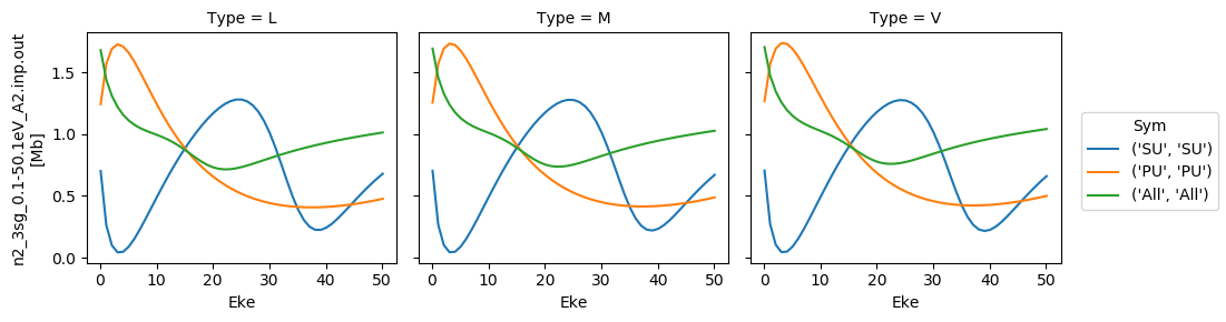
Plot ePS results (isotropic case)
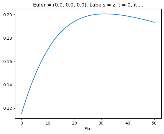
[35]:
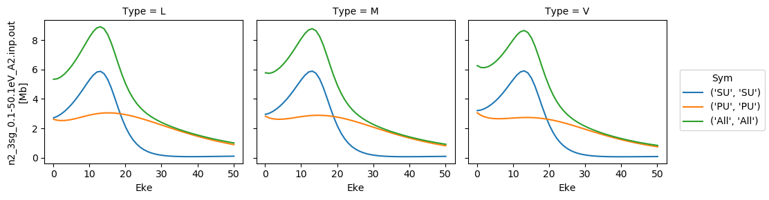
# Plot cross sections using Xarray functionality
# Set here to plot per file - should add some logic to combine files.
for data in dataXS:
    daPlot = data.sel(XC='SIGMA')
    daPlot.plot.line(x='Eke', col='Type')
[35]:
<xarray.plot.facetgrid.FacetGrid at 0x2c402402630>
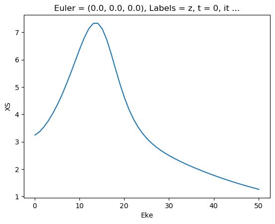
[36]:
# Repeat for betas
for data in dataXS:
    daPlot = data.sel(XC='BETA')
    daPlot.plot.line(x='Eke', col='Type')
[36]:
<xarray.plot.facetgrid.FacetGrid at 0x2c402584828>
Try new AF calculation - isotropic (default) case
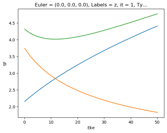
[37]:
# Tabulate & plot matrix elements vs. Eke
selDims = {'it':1, 'Type':'L'}
matE = dataSet[0].sel(selDims)  # Set for N2 case, length-gauge results only.
daPlot, daPlotpd, legendList, gFig = ep.lmPlot(matE, xDim = 'Eke', pType = 'r', fillna = True)
daPlotpd
Plotting data n2_3sg_0.1-50.1eV_A2.inp.out, pType=r, thres=0.01, with Seaborn
[37]:
| Eke | 0.1 | 1.1 | 2.1 | 3.1 | 4.1 | 5.1 | 6.1 | 7.1 | 8.1 | 9.1 | ... | 41.1 | 42.1 | 43.1 | 44.1 | 45.1 | 46.1 | 47.1 | 48.1 | 49.1 | 50.1 | |||||
|---|---|---|---|---|---|---|---|---|---|---|---|---|---|---|---|---|---|---|---|---|---|---|---|---|---|---|
| Cont | Targ | Total | l | m | mu | |||||||||||||||||||||
| PU | SG | PU | 1 | -1 | 1 | -6.203556 | 7.496908 | 3.926892 | 1.071093 | -0.335132 | -1.043391 | -1.396885 | -1.554984 | -1.598812 | -1.573327 | ... | -0.396306 | -0.422225 | -0.448003 | -0.473466 | -0.498463 | -0.522867 | -0.546573 | -0.569493 | -0.591558 | -0.612712 |
| 1 | -1 | -6.203556 | 7.496908 | 3.926892 | 1.071093 | -0.335132 | -1.043391 | -1.396885 | -1.554984 | -1.598812 | -1.573327 | ... | -0.396306 | -0.422225 | -0.448003 | -0.473466 | -0.498463 | -0.522867 | -0.546573 | -0.569493 | -0.591558 | -0.612712 | ||||
| 3 | -1 | 1 | -2.090641 | -1.723467 | -3.571018 | -1.703191 | 0.232612 | 1.862713 | 3.201022 | 4.298839 | 5.198215 | 5.929303 | ... | 1.200463 | 1.040074 | 0.892501 | 0.757189 | 0.633556 | 0.521004 | 0.418928 | 0.326726 | 0.243800 | 0.169566 | |||
| 1 | -1 | -2.090641 | -1.723467 | -3.571018 | -1.703191 | 0.232612 | 1.862713 | 3.201022 | 4.298839 | 5.198215 | 5.929303 | ... | 1.200463 | 1.040074 | 0.892501 | 0.757189 | 0.633556 | 0.521004 | 0.418928 | 0.326726 | 0.243800 | 0.169566 | ||||
| 5 | -1 | 1 | 0.000000 | 0.013246 | 0.000000 | -0.013096 | -0.024367 | -0.033455 | -0.042762 | -0.053765 | -0.067354 | -0.083946 | ... | -0.325544 | -0.318791 | -0.312332 | -0.306211 | -0.300456 | -0.295091 | -0.290130 | -0.285584 | -0.281453 | -0.277737 | |||
| 1 | -1 | 0.000000 | 0.013246 | 0.000000 | -0.013096 | -0.024367 | -0.033455 | -0.042762 | -0.053765 | -0.067354 | -0.083946 | ... | -0.325544 | -0.318791 | -0.312332 | -0.306211 | -0.300456 | -0.295091 | -0.290130 | -0.285584 | -0.281453 | -0.277737 | ||||
| 7 | -1 | 1 | 0.000000 | 0.000000 | 0.000000 | 0.000000 | 0.000000 | 0.000000 | 0.000000 | 0.000000 | 0.000000 | 0.000000 | ... | 0.027469 | 0.028083 | 0.028678 | 0.029257 | 0.029823 | 0.030377 | 0.030923 | 0.031461 | 0.031994 | 0.032523 | |||
| 1 | -1 | 0.000000 | 0.000000 | 0.000000 | 0.000000 | 0.000000 | 0.000000 | 0.000000 | 0.000000 | 0.000000 | 0.000000 | ... | 0.027469 | 0.028083 | 0.028678 | 0.029257 | 0.029823 | 0.030377 | 0.030923 | 0.031461 | 0.031994 | 0.032523 | ||||
| SU | SG | SU | 1 | 0 | 0 | 6.246520 | -10.081763 | -8.912214 | -5.342049 | -3.160539 | -1.795783 | -0.867993 | -0.174154 | 0.400643 | 0.926420 | ... | -0.854886 | -0.940017 | -1.021577 | -1.099776 | -1.174787 | -1.246759 | -1.315814 | -1.382058 | -1.445582 | -1.506467 |
| 3 | 0 | 0 | 2.605768 | 2.775108 | 4.733473 | 1.677812 | -1.450830 | -4.187395 | -6.554491 | -8.601759 | -10.343109 | -11.747922 | ... | -0.293053 | -0.441416 | -0.579578 | -0.708075 | -0.827415 | -0.938075 | -1.040506 | -1.135134 | -1.222361 | -1.302566 | |||
| 5 | 0 | 0 | 0.000000 | -0.020864 | 0.000000 | 0.024263 | 0.042694 | 0.059142 | 0.077308 | 0.099330 | 0.126227 | 0.157745 | ... | 0.490499 | 0.511546 | 0.531810 | 0.551281 | 0.569951 | 0.587815 | 0.604868 | 0.621107 | 0.636528 | 0.651132 | |||
| 7 | 0 | 0 | 0.000000 | 0.000000 | 0.000000 | 0.000000 | 0.000000 | 0.000000 | 0.000000 | 0.000000 | 0.000000 | 0.000000 | ... | -0.039566 | -0.041422 | -0.043265 | -0.045092 | -0.046901 | -0.048689 | -0.050453 | -0.052190 | -0.053899 | -0.055577 |
12 rows × 51 columns
[38]:
phaseConvention = 'E'  # Set phase conventions used in the numerics - for ePolyScat matrix elements, set to 'E', to match defns. above.

symSum = False  # Sum over symmetry groups, or keep separate?
SFflag = True  # Include scaling factor to Mb in calculation?
thres = 1e-4
RX = ep.setPolGeoms()  # Set default pol geoms (z,x,y), or will be set by mfblmXprod() defaults - FOR AF case this is only used to set 'z' geom for unity wigner D's - should rationalise this!

start = time.time()
mTermST, mTermS, mTermTest = ep.geomFunc.afblmXprod(dataSet[0], QNs = None, RX=RX, thres = thres, selDims = {'it':1, 'Type':'L'}, thresDims='Eke', symSum=symSum, SFflag=True, phaseConvention=phaseConvention)
end = time.time()
print('Elapsed time = {0} seconds, for {1} energy points, {2} polarizations, threshold={3}.'.format((end-start), mTermST.Eke.size, RX.size, thres))

# Elapsed time = 3.3885273933410645 seconds, for 51 energy points, 3 polarizations, threshold=0.01.
# Elapsed time = 5.059587478637695 seconds, for 51 energy points, 3 polarizations, threshold=0.0001.
Elapsed time = 2.529463768005371 seconds, for 51 energy points, 3 polarizations, threshold=0.0001.
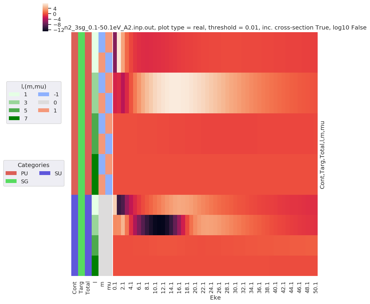
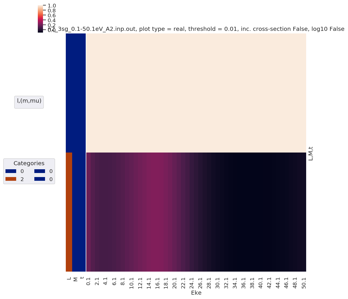
[39]:
# Full results (before summation)
mTermST.attrs['dataType'] = 'matE'  # Set matE here to allow for correct plotting of sym dims.

plotDimsRed = ['Labels','L','M']  # Set plotDims to fix dim ordering in plot
if not symSum:
    plotDimsRed.extend(['Cont','Targ','Total'])

daPlot, daPlotpd, legendList, gFig = ep.lmPlot(mTermST, plotDims=plotDimsRed, xDim='Eke', sumDims=None, pType = 'r', thres = 0.01, fillna = True, SFflag=False)

# daPlot, daPlotpd, legendList, gFig = ep.lmPlot(mTermST, xDim='Eke', sumDims=None, pType = 'r', thres = 0.01, fillna = True)  # If plotDims is not passed use default ordering.
Plotting data n2_3sg_0.1-50.1eV_A2.inp.out, pType=r, thres=0.01, with Seaborn
No handles with labels found to put in legend.
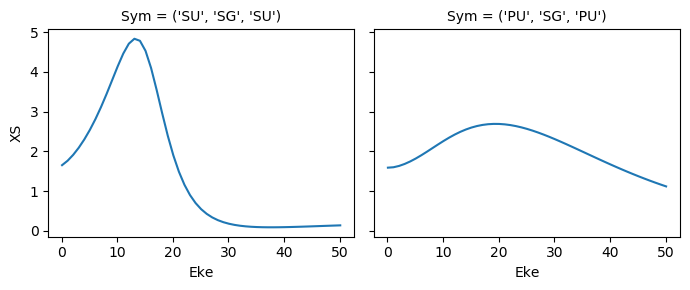
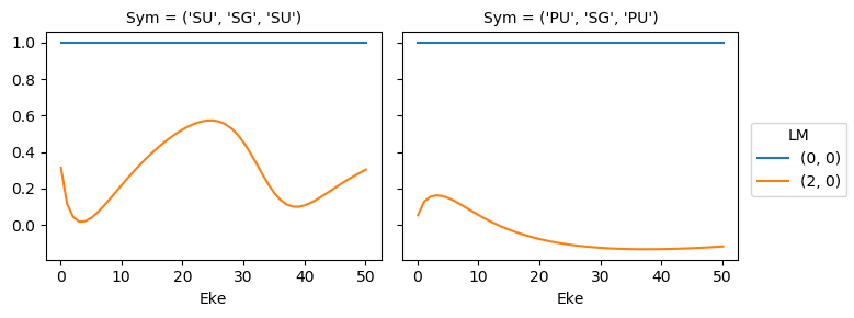
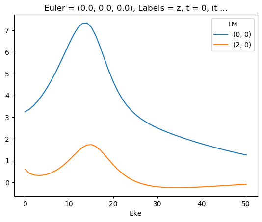
[40]:
mTermST.XS.real.squeeze().plot.line(x='Eke', col='Sym');
ep.util.matEleSelector(mTermST, thres = 0.1, dims='Eke').real.squeeze().plot.line(x='Eke', col='Sym');
Try sym summation…
[41]:
phaseConvention = 'E'  # Set phase conventions used in the numerics - for ePolyScat matrix elements, set to 'E', to match defns. above.

symSum = True  # Sum over symmetry groups, or keep separate?
SFflag = True  # Include scaling factor to Mb in calculation?
thres = 1e-4
RX = ep.setPolGeoms()  # Set default pol geoms (z,x,y), or will be set by mfblmXprod() defaults - FOR AF case this is only used to set 'z' geom for unity wigner D's - should rationalise this!

start = time.time()
mTermST, mTermS, mTermTest = ep.geomFunc.afblmXprod(dataSet[0], QNs = None, RX=RX, thres = thres, selDims = {'it':1, 'Type':'L'}, thresDims='Eke', symSum=symSum, SFflag=SFflag, phaseConvention=phaseConvention)
end = time.time()
print('Elapsed time = {0} seconds, for {1} energy points, {2} polarizations, threshold={3}.'.format((end-start), mTermST.Eke.size, RX.size, thres))

# Elapsed time = 3.3885273933410645 seconds, for 51 energy points, 3 polarizations, threshold=0.01.
# Elapsed time = 5.059587478637695 seconds, for 51 energy points, 3 polarizations, threshold=0.0001.
Elapsed time = 2.300682306289673 seconds, for 51 energy points, 3 polarizations, threshold=0.0001.
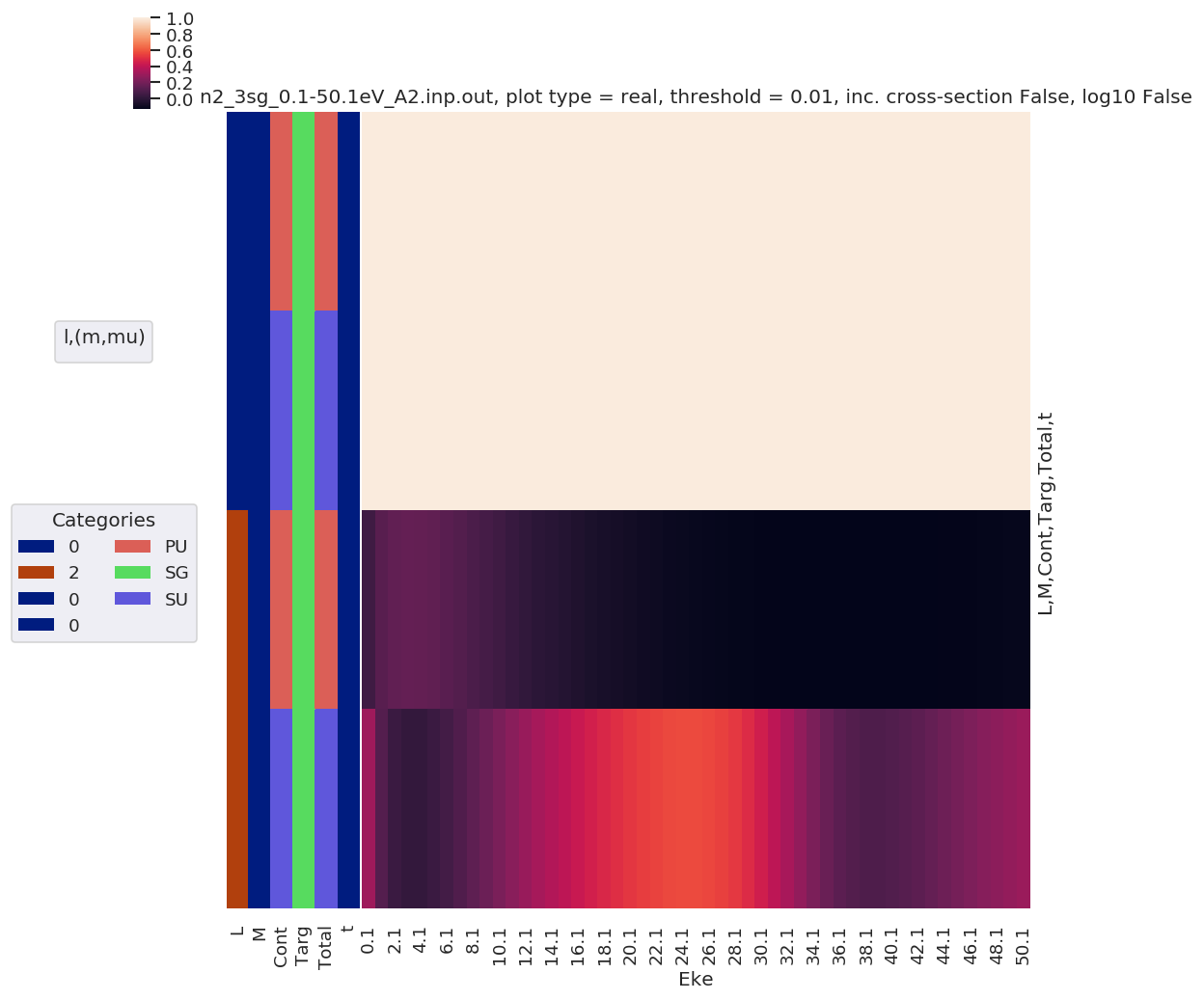
[42]:
# Full results (before summation)
mTermST.attrs['dataType'] = 'matE'  # Set matE here to allow for correct plotting of sym dims.

plotDimsRed = ['Labels','L','M']  # Set plotDims to fix dim ordering in plot
if not symSum:
    plotDimsRed.extend(['Cont','Targ','Total'])

daPlot, daPlotpd, legendList, gFig = ep.lmPlot(mTermST, plotDims=plotDimsRed, xDim='Eke', sumDims=None, pType = 'r', thres = 0.01, fillna = True, SFflag=False)

# daPlot, daPlotpd, legendList, gFig = ep.lmPlot(mTermST, xDim='Eke', sumDims=None, pType = 'r', thres = 0.01, fillna = True)  # If plotDims is not passed use default ordering.
Plotting data n2_3sg_0.1-50.1eV_A2.inp.out, pType=r, thres=0.01, with Seaborn
No handles with labels found to put in legend.
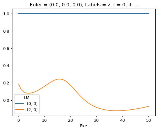
[43]:
mTermST.XS.real.squeeze().plot.line(x='Eke');

[44]:
ep.util.matEleSelector(mTermST, thres = 0.1, dims='Eke').real.squeeze().plot.line(x='Eke');
First attempt… with sym summation
Looks quite different - might be SF issue with combining continua, and/or degen factor…?
Looks same as previous AF code attempt (http://localhost:8888/lab/tree/dev/ePSproc/ePSproc_AFBLM_calcs_bench_100220.ipynb), suggesting something in degen/normalisation in formalism amiss?
[45]:
# ep.util.matEleSelector(mTermST, thres = 0.1, dims='Eke').real.squeeze().plot.line(x='Eke');
ep.util.matEleSelector(mTermST, thres = 0.1, dims='Eke').imag.squeeze().plot.line(x='Eke');
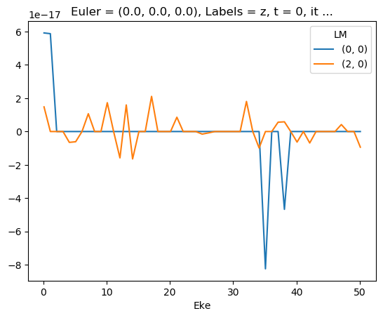
Test mult and renorm - seems like E-dependent XS issue here…
[ ]:
[46]:
mTermTest = mTermST.copy()
# mTermTest.values = mTermTest*mTermTest.SF
# mTermTest.values = mTermTest/mTermTest.SF.pipe(np.abs)
mTermTest.values = mTermTest/mTermTest.SF
ep.util.matEleSelector(mTermTest, thres = 0.1, dims='Eke').real.squeeze().plot.line(x='Eke');
[47]:
ep.util.matEleSelector(mTermST['XS'], thres = 0.1, dims='Eke').real.squeeze().plot.line(x='Eke');
[48]:
ep.util.matEleSelector(mTermST['SF'], thres = 0.1, dims='Eke').real.squeeze().plot.line(x='Eke');
ep.util.matEleSelector(mTermST['SF'], thres = 0.1, dims='Eke').imag.squeeze().plot.line(x='Eke');
ep.util.matEleSelector(mTermST['SF'], thres = 0.1, dims='Eke').pipe(np.abs).squeeze().plot.line(x='Eke');
[49]:
mTermST.values = mTermST*mTermST.XS
ep.util.matEleSelector(mTermST, thres = 0.1, dims='Eke').real.squeeze().plot.line(x='Eke');
[50]:
matE.values = matE * matE.SF
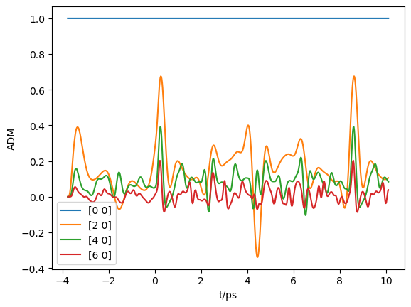
Test compared to experimental N2 AF results…
In this case MF PADs look good, so also expect good agreement with AF…
[51]:
# Adapted from ePSproc_AFBLM_testing_010519_300719.m
# Load ADMs for N2
from scipy.io import loadmat
ADMdataFile = os.path.join(modPath, 'data', 'alignment', 'N2_ADM_VM_290816.mat')
ADMs = loadmat(ADMdataFile)
[52]:
# Set tOffset for calcs, 3.76ps!!!
# This is because this is 2-pulse case, and will set t=0 to 2nd pulse (and matches defn. in N2 experimental paper)
tOffset = -3.76
ADMs['time'] = ADMs['time'] + tOffset
[53]:
# Plot
import matplotlib.pyplot as plt
plt.plot(ADMs['time'].T, np.real(ADMs['ADM'].T))
plt.legend(ADMs['ADMlist'])
plt.xlabel('t/ps')
plt.ylabel('ADM')
plt.show()
[53]:
[<matplotlib.lines.Line2D at 0x2c40580a0b8>,
 <matplotlib.lines.Line2D at 0x2c4007392e8>,
 <matplotlib.lines.Line2D at 0x2c400cc70f0>,
 <matplotlib.lines.Line2D at 0x2c400cc7f28>]
[53]:
<matplotlib.legend.Legend at 0x2c400960828>
[53]:
Text(0.5, 0, 't/ps')
[53]:
Text(0, 0.5, 'ADM')
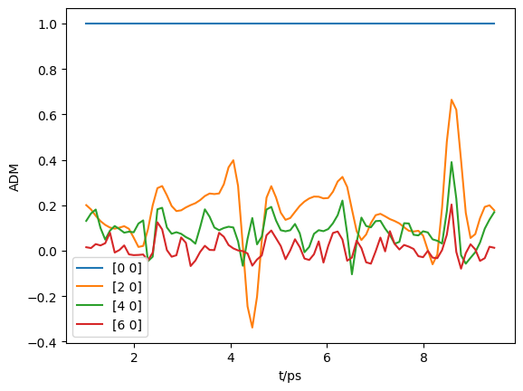
[54]:
# Selection & downsampling
trange=[1, 9.5]  # Set range in ps for calc
tStep=5  # Set tStep for downsampling

tMask = (ADMs['time']>trange[0]) * (ADMs['time']<trange[1])
ind = np.nonzero(tMask)[1][0::tStep]
At = ADMs['time'][:,ind].squeeze()
ADMin = ADMs['ADM'][:,ind]

print(f"Selecting {ind.size} points")

plt.plot(At, np.real(ADMin.T))
plt.legend(ADMs['ADMlist'])
plt.xlabel('t/ps')
plt.ylabel('ADM')
plt.show()

# Set in Xarray
ADMX = ep.setADMs(ADMs = ADMs['ADM'][:,ind], t=At, KQSLabels = ADMs['ADMlist'], addS = True)
# ADMX
Selecting 87 points
[54]:
[<matplotlib.lines.Line2D at 0x2c400b3b080>,
 <matplotlib.lines.Line2D at 0x2c4724dea20>,
 <matplotlib.lines.Line2D at 0x2c400b4f2e8>,
 <matplotlib.lines.Line2D at 0x2c400b4f208>]
[54]:
<matplotlib.legend.Legend at 0x2c4024c6908>
[54]:
Text(0.5, 0, 't/ps')
[54]:
Text(0, 0.5, 'ADM')
[73]:
# Run with sym summation...

phaseConvention = 'E'  # Set phase conventions used in the numerics - for ePolyScat matrix elements, set to 'E', to match defns. above.

symSum = True  # Sum over symmetry groups, or keep separate?
SFflag = False  # Include scaling factor to Mb in calculation?
BLMRenorm = False
thres = 1e-4
RX = ep.setPolGeoms()  # Set default pol geoms (z,x,y), or will be set by mfblmXprod() defaults - FOR AF case this is only used to set 'z' geom for unity wigner D's - should rationalise this!

start = time.time()
mTermST, mTermS, mTermTest = ep.geomFunc.afblmXprod(dataSet[0], QNs = None, AKQS=ADMX, RX=RX, thres = thres, selDims = {'it':1, 'Type':'L'}, thresDims='Eke',
                                                    symSum=symSum, SFflag=SFflag, BLMRenorm = BLMRenorm,
                                                    phaseConvention=phaseConvention)
end = time.time()
print('Elapsed time = {0} seconds, for {1} energy points, {2} polarizations, threshold={3}.'.format((end-start), mTermST.Eke.size, RX.size, thres))

# Elapsed time = 3.3885273933410645 seconds, for 51 energy points, 3 polarizations, threshold=0.01.
# Elapsed time = 5.059587478637695 seconds, for 51 energy points, 3 polarizations, threshold=0.0001.
Elapsed time = 3.8453733921051025 seconds, for 51 energy points, 3 polarizations, threshold=0.0001.
[74]:
# Full results (before summation)
mTermST.attrs['dataType'] = 'matE'  # Set matE here to allow for correct plotting of sym dims.

plotDimsRed = ['Labels','L','M']  # Set plotDims to fix dim ordering in plot
if not symSum:
    plotDimsRed.extend(['Cont','Targ','Total'])

# daPlot, daPlotpd, legendList, gFig = ep.lmPlot(mTermST, plotDims=plotDimsRed, xDim='Eke', sumDims=None, pType = 'r', thres = 0.01, fillna = True, SFflag=False)

# daPlot, daPlotpd, legendList, gFig = ep.lmPlot(mTermST, xDim='Eke', sumDims=None, pType = 'r', thres = 0.01, fillna = True)  # If plotDims is not passed use default ordering.
[75]:
# daPlot, daPlotpd, legendList, gFig = ep.lmPlot(mTermST.XS, plotDims=plotDimsRed, xDim='Eke', sumDims=None, pType = 'r', thres = 0.01, fillna = True, SFflag=False)
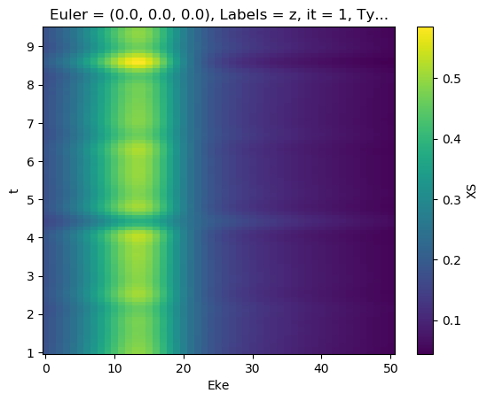
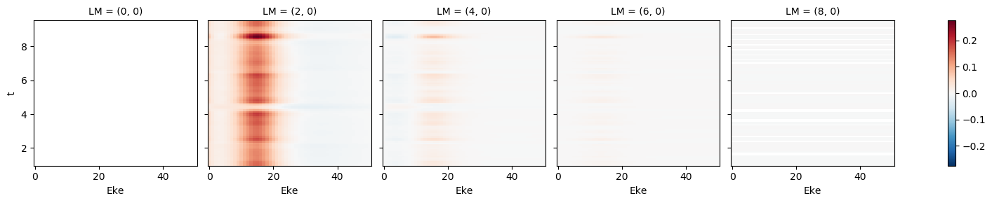
[76]:
mTermST.XS.real.plot()
mTermST.where(mTermST.L > 0).real.plot(col='LM')
[76]:
<matplotlib.collections.QuadMesh at 0x2c400c7a0b8>
[76]:
<xarray.plot.facetgrid.FacetGrid at 0x2c4058c19e8>
[77]:
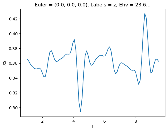
# Plot single energy XS
E = 8.1
mTermST.XS.sel({'Eke':E}).real.squeeze().plot.line(x='t');
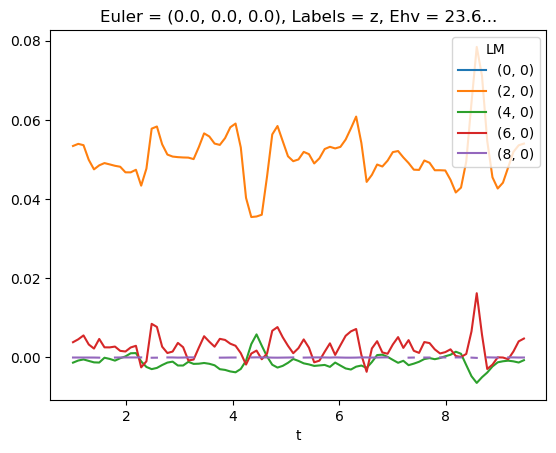
[78]:
# LM with renorm
mTermST.sel({'Eke':E}).where(mTermST['L']>0).real.squeeze().plot.line(x='t');
[72]:
# LM * XS
# (mTermST * mTermST.XS).sel({'Eke':E}).where(mTermST['L']>0).real.squeeze().plot.line(x='t');
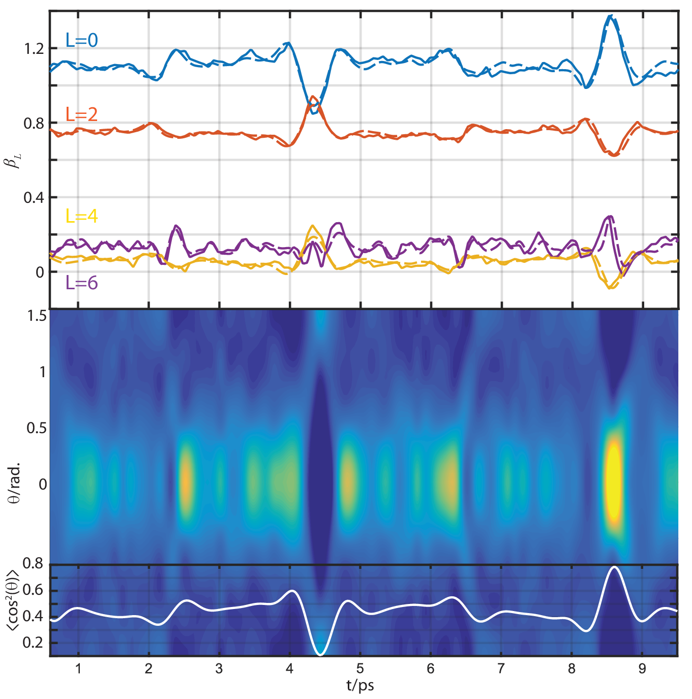
Experimental results
(Fig 2 from Marceau, Claude, Varun Makhija, Dominique Platzer, A. Yu. Naumov, P. B. Corkum, Albert Stolow, D. M. Villeneuve, and Paul Hockett. “Molecular Frame Reconstruction Using Time-Domain Photoionization Interferometry.” Physical Review Letters 119, no. 8 (August 2017): 083401. https://doi.org/10.1103/PhysRevLett.119.083401. Full data at https://doi.org/10.6084/m9.figshare.4480349.v10)
Currently:
Relative signs/phases of betas look good at 4.1eV… but not at 7.1 or 8.1eV! (Experimental MFPAD comparison energy) - suggests still phase and/or renorm issue somewhere?
Values still off, same issue probably.
Might be phase issue with sum over rotation matrix elements, which are conj() in MF case, but not in original derivation here…? This could give 3j sign-flip, hence change calculated alignment response.
SCRATCH
[62]:
# Phase switch example
        if phaseCons['mfblmCons']['BLMmPhase']:
            QNsBLMtable[:,3] *= -1
            QNsBLMtable[:,5] *= -1
  File "<ipython-input-62-6783c300192b>", line 2
    if phaseCons['mfblmCons']['BLMmPhase']:
    ^
IndentationError: unexpected indent
[ ]:
def deltaKQS(QNs = None):
    phaseCons = setPhaseConventions(phaseConvention = phaseConvention)

    # If no QNs are passed, set for all possible terms
    if QNs is None:
        QNs = []

        # Set photon terms
        l = 1
        lp = 1

        # Loop to set all other QNs
        for mu in np.arange(-l, l+1):
            for mup in np.arange(-lp, lp+1):
                #for R in np.arange(-(l+lp)-1, l+lp+2):
                #    for P in np.arange(0, l+lp+1):
                for P in np.arange(0, l+lp+1):
                    # for Rp in np.arange(-P, P+1):  # Allow all Rp
                    # Rp = -(mu+mup)   # Fix Rp terms - not valid here, depends on other phase cons!
                    # for R in np.arange(-P, P+1):
                    #     # QNs.append([l, lp, P, mu, -mup, R, Rp])
                    #     if phaseCons['lambdaCons']['negRp']:
                    #         Rp *= -1
                    #     if phaseCons['lambdaCons']['negMup']:
                    #         QNs.append([l, lp, P, mu, -mup, Rp, R])   # 31/03/20: FIXED bug, (R,Rp) previously misordered!!!
                    #     else:
                    #         QNs.append([l, lp, P, mu, mup, Rp, R])

                    # Rearranged for specified Rp case
                    for R in np.arange(-P, P+1):
                        # if phaseCons['lambdaCons']['negMup']:
                        #     mup = -mup

                        if phaseCons['lambdaCons']['negRp']:
                            # Rp = mu+mup
                            Rp = mup - mu
                        else:
                            Rp = -(mu+mup)

                        # Switch mup sign for 3j?  To match old numerics, this is *after* Rp assignment (sigh).
                        if phaseCons['lambdaCons']['negMup']:
                            mup = -mup

                        QNs.append([l, lp, P, mu, mup, Rp, R])

        QNs = np.array(QNs)