Working with real spherical harmonics
20/09/22
This notebook gives a brief introduction to some of the conventions and functionality for handling real spherical harmonics and related functions, using low-level ePSproc routines. For complex spherical harmonics, and more general method notes, see ‘working with complex harmonics’ - note the complex forms are generally used in ePSproc, and general correct handling for cases using real spherical harmonics is not currently implemented/guaranteed.
Note some higher-level routines are available in the base class.
Definitions
Per the Wikipaedia definitions, the real spherical harmonics can be defined as:
Where \(Y_{\ell m}\) are real harmonics, and \(Y_{\ell }^{m}\) are complex.
And the inverse relations:
The real harmonics can also be written explicitly as:
For futher information, see wikipeadia or the SHtools introduction to real spherical harmonics.
Numerical implementation
ePSproc currently (Sept. 2022) implements:
Generation of real harmonics.
Conversion of real harmonic coefficients to complex harmonic coefficients.
General handling for real spherical harmonics is not guaranteed however, although - as per above - they can be defined simply by suitable combinations of complex harmonics. Note that the default routines in ePSproc make use of scipy.special.sph_harm as the default calculation routine, this is implemented with a default \((\theta, \phi)\) definition, and normalisation, corresponding to the usual “physics” convention (\(\theta\) defined from the z-axis, includes the Condon-Shortley phase, and orthonormalised). See ‘working with complex harmonics’ for further discussion; the real harmonics are then defined from the complex forms following the final definition given above, where the Condon-Shortley phase is already included in the \(Y_{\ell }^{|m|}\) terms:
(For a basic python routine, see Visualizing the real forms of the spherical harmonics.)
Imports
[1]:
import xarray as xr
import pandas as pd
import numpy as np
import epsproc as ep
# Set compact XR repr
xr.set_options(display_expand_data = False)
OMP: Info #273: omp_set_nested routine deprecated, please use omp_set_max_active_levels instead.
* sparse not found, sparse matrix forms not available.
* natsort not found, some sorting functions not available.
* Hvplot not found, some hvPlotters may not be available. See https://hvplot.holoviz.org/user_guide/Gridded_Data.html for package details.
* Setting plotter defaults with epsproc.basicPlotters.setPlotters(). Run directly to modify, or change options in local env.


* Set Holoviews with bokeh.
* pyevtk not found, VTK export not available.
[1]:
<xarray.core.options.set_options at 0x7f879072f400>
Computing spherical harmonics on a grid
A basic wrapper for the backends is provided by ep.sphCalc. This computes spherical harmonics for all orders up to Lmax, for a given angular resolution or set of angles, and returns an Xarray. Set fnType = 'real' for real harmonics.
[2]:
# Compute harmonics for 50x50 (theta,phi) grid
Ire = ep.sphCalc(Lmax = 2, res = 50, fnType = 'real')
Ire
[2]:
<xarray.DataArray 'YLM' (LM: 9, Phi: 50, Theta: 50)>
0.2821 0.2821 0.2821 0.2821 0.2821 ... 0.03515 0.01996 0.008933 0.002242 0.0
Coordinates:
* LM (LM) object MultiIndex
* l (LM) int64 0 1 1 1 2 2 2 2 2
* m (LM) int64 0 -1 0 1 -2 -1 0 1 2
* Phi (Phi) float64 0.0 0.1282 0.2565 0.3847 ... 5.899 6.027 6.155 6.283
* Theta (Theta) float64 0.0 0.06411 0.1282 0.1923 ... 3.013 3.077 3.142
Attributes:
dataType: YLM
long_name: Spherical harmonics
harmonics: {'dtype': 'Real harmonics', 'kind': 'real', 'normType': 'orth...
units: arb[3]:
# Plot some components
# Ire = ep.sphCalc(Lmax = 2, res = 50, fnType = 'real')
ep.sphSumPlotX(Ire.sel(l=2), facetDim = 'm', backend = 'pl');
*** WARNING: plot dataset has min value < 0, min = -0.5459935484542385. This may be unphysical and/or result in plotting issues.
Sph plots:
Plotting with facetDims=m, pType=a with backend=pl.
*** Plotting for [1,1,0]
*** Plotting for [1,2,1]
*** Plotting for [1,3,2]
*** Plotting for [1,4,3]
*** Plotting for [1,5,4]
[4]:
# Compare with complex case (default)
IC = ep.sphCalc(Lmax = 2, res = 50)
ep.sphSumPlotX(IC.sel(l=2), facetDim = 'm', backend = 'pl', titleString='Abs');
ep.sphSumPlotX(IC.sel(l=2), facetDim = 'm', backend = 'pl', pType = 'r', titleString='Real component');
ep.sphSumPlotX(IC.sel(l=2), facetDim = 'm', backend = 'pl', pType = 'i', titleString='Imaginary component');
*** WARNING: plot dataset has min value < 0, min = (-0.38607574059609784-9.456128398989102e-17j). This may be unphysical and/or result in plotting issues.
Sph plots: Abs
Plotting with facetDims=m, pType=a with backend=pl.
*** Plotting for [1,1,0]
*** Plotting for [1,2,1]
*** Plotting for [1,3,2]
*** Plotting for [1,4,3]
*** Plotting for [1,5,4]
*** WARNING: plot dataset has min value < 0, min = (-0.38607574059609784-9.456128398989102e-17j). This may be unphysical and/or result in plotting issues.
Sph plots: Real component
Plotting with facetDims=m, pType=r with backend=pl.
*** Plotting for [1,1,0]
*** Plotting for [1,2,1]
*** Plotting for [1,3,2]
*** Plotting for [1,4,3]
*** Plotting for [1,5,4]
*** WARNING: plot dataset has min value < 0, min = (-0.38607574059609784-9.456128398989102e-17j). This may be unphysical and/or result in plotting issues.
Sph plots: Imaginary component
Plotting with facetDims=m, pType=i with backend=pl.
*** Plotting for [1,1,0]
*** Plotting for [1,2,1]
*** Plotting for [1,3,2]
*** Plotting for [1,4,3]
*** Plotting for [1,5,4]
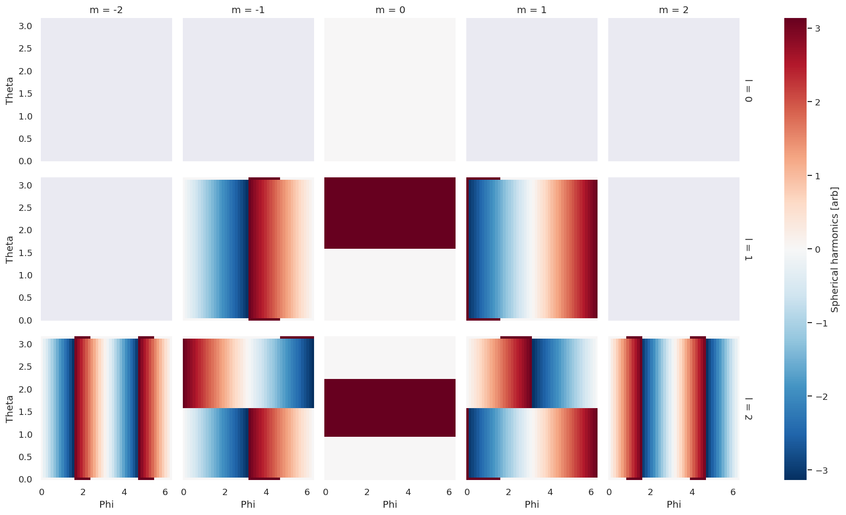
Note that the complex harmonics have rotations between the real and imaginary components, and produce a cylindrically-symmetric absolute valued map (here computed as np.abs(I) \(=\sqrt(a^2+b^2)\) for the complex case \(Z=a+ib\)), whilst the real harmonics have rotations between + and - m pairs.
In general this can be viewed as a phase rotation in the complex plane; this can be visualised more directly by looking at a phase map, which - by definition for the individual components - is given by the term \(e^{im\phi}\). (For summations over sets of harmonics this becomes more interesting!)
[5]:
# Visualise the phase
ep.plotTypeSelector(IC.unstack('LM'), pType = 'phase').plot(y='Theta', x='Phi', row='l', col='m', robust=True)
[5]:
<xarray.plot.facetgrid.FacetGrid at 0x7f8790788370>
Setting coefficients
To manually set coefficients from lists or arrays, use the setBLMs() function, including kind='real' to specify an expansion in real harmonics. These can be used and expanded directly, or via the sphFromBLMPlot() function.
[6]:
# Set all allowed BLM up to Lmax with genLM, random value case
from epsproc.sphCalc import setBLMs
LM = ep.genLM(2)
BLMallrand = setBLMs(np.random.random(LM.shape[0]), LM, kind = 'real')
BLMallrand
[6]:
<xarray.DataArray 'BLM' (BLM: 9, t: 1)>
0.1199 0.03737 0.9135 0.4958 0.2089 0.8747 0.6591 0.1246 0.03624
Coordinates:
* BLM (BLM) object MultiIndex
* l (BLM) int64 0 1 1 1 2 2 2 2 2
* m (BLM) int64 0 -1 0 1 -2 -1 0 1 2
* t (t) int64 0
Attributes:
dataType: BLM
long_name: Beta parameters
units: arb
harmonics: {'dtype': 'Real harmonics', 'kind': 'real', 'normType': 'orth...[7]:
# Direct Xarray tensor multiplication - this will correctly handle dimensions if names match.
Irand = BLMallrand.rename({'BLM':'LM'}).squeeze(drop=True) * Ire
# ep.sphSumPlotX(Irand, facetDim = 't') # Note this may need facetDim set explicitly here for non-1D cases
ep.sphSumPlotX(Irand, facetDim=None, backend='pl');
*** WARNING: plot dataset has min value < 0, min = -0.743550843638639. This may be unphysical and/or result in plotting issues.
Sph plots:
Plotting with facetDims=None, pType=a with backend=pl.
*** Plotting for [1,1,0]
[8]:
# Functional form - this returns array, include plotFlag = True to show plot and return a fig handle
Itp, fig = ep.sphFromBLMPlot(BLMallrand.squeeze(), plotFlag = True, backend='pl')
Itp
Using real betas (from BLMX array).
*** WARNING: plot dataset has min value < 0, min = -0.743550843638639. This may be unphysical and/or result in plotting issues.
Sph plots:
Plotting with facetDims=None, pType=a with backend=pl.
*** Plotting for [1,1,0]
[8]:
<xarray.DataArray (LM: 9, Phi: 50, Theta: 50)>
0.03381 0.03381 0.03381 0.03381 0.03381 ... 0.0007233 0.0003237 8.126e-05 0.0
Coordinates:
* LM (LM) object MultiIndex
* l (LM) int64 0 1 1 1 2 2 2 2 2
* m (LM) int64 0 -1 0 1 -2 -1 0 1 2
t int64 0
* Phi (Phi) float64 0.0 0.1282 0.2565 0.3847 ... 5.899 6.027 6.155 6.283
* Theta (Theta) float64 0.0 0.06411 0.1282 0.1923 ... 3.013 3.077 3.142
Attributes:
dataType: Itp
long_name: I(\theta,\phi)
harmonics: {'dtype': 'Real harmonics', 'kind': 'real', 'normType': 'orth...
units: arb
normType: realConverting coefficients real to complex form
Basic conversion is implemented in epsproc.sphFuncs.sphConv.sphRealConvert().
This currently (Sept. 2022) has two methods implemented for conversion:
‘sh’: Set terms as per SHtools definitions, https://shtools.github.io/SHTOOLS/complex-spherical-harmonics.html Note this form has purely real or purely imaginary terms.
‘std’: Set +/-m terms from |m| real harmonics as per wikipedia defn, https://en.wikipedia.org/wiki/Spherical_harmonics#Real_form Note: this form currently assumes only +M or -M for any given term, and also sets conjugates upon conversion if incConj=True. This may be phase-rotated relative to SHtools convention. NOTE: THIS METHOD CURRENTLY FAILS - phase issues somewhere, produces incorrect expansions in complex harmonics.
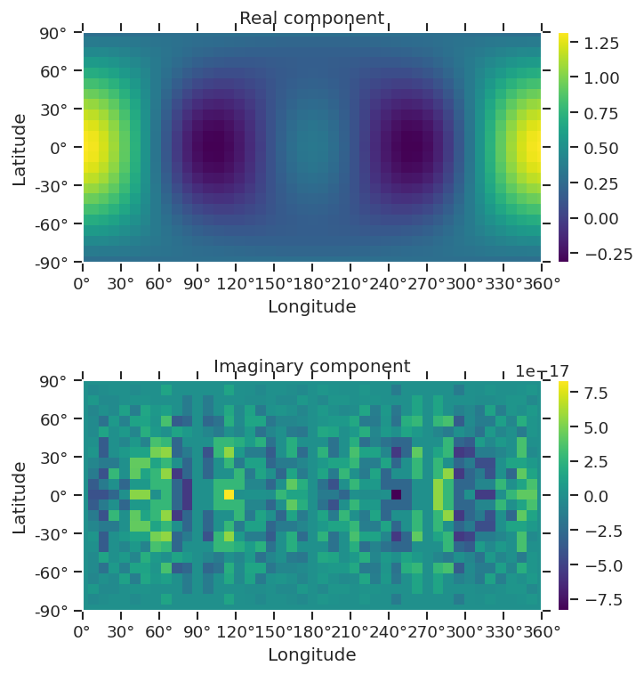
A basic demo is given below. In general, plotting the original and converted forms is a good test of consistency here, and SHtools can also be used directly as an independent method and cross-check (note, however, that this will only work for 1D cases, whilst sphRealConvert() will work accross any N-dimensional Xarray).
[9]:
# Basic distribution
BLM = setBLMs([[0,0,1],[1,1,1],[2,2,1]], kind='real').squeeze(drop=True)
BLM
[9]:
<xarray.DataArray 'BLM' (BLM: 3)>
1 1 1
Coordinates:
* BLM (BLM) object MultiIndex
* l (BLM) int64 0 1 2
* m (BLM) int64 0 1 2
Attributes:
dataType: BLM
long_name: Beta parameters
units: arb
harmonics: {'dtype': 'Real harmonics', 'kind': 'real', 'normType': 'orth...[10]:
backend = 'pl'
ItpRe, fig = ep.sphFromBLMPlot(BLM, plotFlag = True, backend = backend) #, fnType = 'real')
Using real betas (from BLMX array).
*** WARNING: plot dataset has min value < 0, min = -0.31421027069653457. This may be unphysical and/or result in plotting issues.
Sph plots:
Plotting with facetDims=None, pType=a with backend=pl.
*** Plotting for [1,1,0]
[11]:
from epsproc.sphFuncs.sphConv import *
BLMconvSH = sphRealConvert(BLM, method='sh') #, addCSphase = False)
ItpCSH, fig = ep.sphFromBLMPlot(BLMconvSH, plotFlag = True, backend = backend, pType='a')
BLMconvSH
Using complex betas (from BLMX array).
*** WARNING: plot dataset has min value < 0, min = (-0.3142102706965345+0j). This may be unphysical and/or result in plotting issues.
Sph plots:
Plotting with facetDims=None, pType=a with backend=pl.
*** Plotting for [1,1,0]
[11]:
<xarray.DataArray 'BLM' (BLM: 5)>
(1+0j) (-0.7071067811865475-0j) ... (0.7071067811865475+0j)
Coordinates:
* BLM (BLM) object MultiIndex
* l (BLM) int64 0 1 1 2 2
* m (BLM) int64 0 -1 1 -2 2
Attributes:
dataType: BLM
long_name: Beta parameters
units: arb
harmonics: {'dtype': 'Complex harmonics', 'kind': 'complex', 'normType':...SHtools conversion & plots
[20]:
# Check vs. shtools routine
# Create SHtools object - note some additional settings may need to be specified
sh = SHcoeffsFromXR(BLM) #, kind = 'real')
shC = sh.convert(kind = 'complex') #, csphase =1 , normalization='4pi') # Optional conversion options, will be taken from BLM.attrs['harmonics'] if not set
shC
[20]:
kind = 'complex'
normalization = 'ortho'
csphase = 1
lmax = 2
error_kind = None
header = None
header2 = None
name = None
units = None
[12]:
# shC.coeffs # Display array
tabulateLM(XRcoeffsFromSH(shC)) # Display table
[12]:
| m | -2 | -1 | 0 | 1 | 2 |
|---|---|---|---|---|---|
| l | |||||
| 0 | 0.000000+0.000000j | 0.000000+0.000000j | 1.0+0.0j | 0.000000+0.000000j | 0.000000+0.000000j |
| 1 | 0.000000+0.000000j | -0.707107+0.000000j | 0.0+0.0j | 0.707107+0.000000j | 0.000000+0.000000j |
| 2 | 0.707107-0.000000j | 0.000000+0.000000j | 0.0+0.0j | 0.000000+0.000000j | 0.707107+0.000000j |
[13]:
# Compare params directly - looks good
tabulateLM(BLMconvSH)
[13]:
| m | -2 | -1 | 0 | 1 | 2 |
|---|---|---|---|---|---|
| l | |||||
| 0 | 0.000000+0.000000j | 0.000000+0.000000j | 1.0+0.0j | 0.000000+0.000000j | 0.000000+0.000000j |
| 1 | 0.000000+0.000000j | -0.707107-0.000000j | 0.0+0.0j | 0.707107+0.000000j | 0.000000+0.000000j |
| 2 | 0.707107-0.000000j | 0.000000+0.000000j | 0.0+0.0j | 0.000000+0.000000j | 0.707107+0.000000j |
[14]:
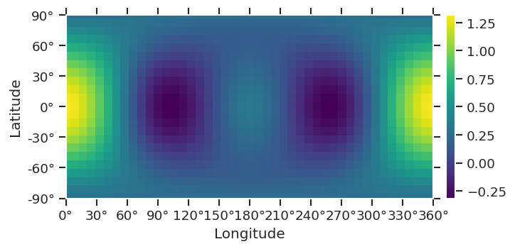
# Plot maps with SHtools
# Original REAL case
# SHtools expand on grid & plot
lmaxGrid = 10
grid = sh.expand(lmax = lmaxGrid)
grid.plot(colorbar='right')
[14]:
(<Figure size 720x360 with 2 Axes>,
<AxesSubplot:xlabel='Longitude', ylabel='Latitude'>)
[15]:
# SHtools real > complex case
grid = shC.expand(lmax = lmaxGrid)
grid.plot(colorbar='right')
[15]:
(<Figure size 720x792 with 4 Axes>,
array([<AxesSubplot:title={'center':'Real component'}, xlabel='Longitude', ylabel='Latitude'>,
<AxesSubplot:title={'center':'Imaginary component'}, xlabel='Longitude', ylabel='Latitude'>],
dtype=object))
[16]:
# Test vs. ePSproc conversion
shC2 = SHcoeffsFromXR(BLMconvSH)
grid = shC2.expand(lmax = lmaxGrid)
grid.plot(colorbar='right')
[16]:
(<Figure size 720x792 with 4 Axes>,
array([<AxesSubplot:title={'center':'Real component'}, xlabel='Longitude', ylabel='Latitude'>,
<AxesSubplot:title={'center':'Imaginary component'}, xlabel='Longitude', ylabel='Latitude'>],
dtype=object))
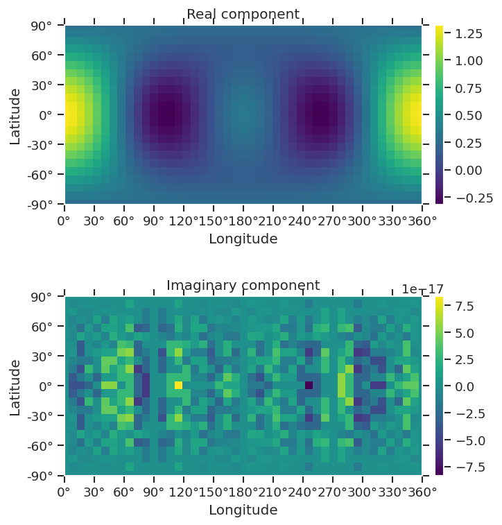
Looks good.
Versions
[17]:
import scooby
scooby.Report(additional=['epsproc', 'holoviews', 'hvplot', 'xarray', 'matplotlib', 'bokeh'])
[17]:
| Thu Sep 29 15:23:21 2022 UTC | |||||||
| OS | Linux | CPU(s) | 32 | Machine | x86_64 | Architecture | 64bit |
| RAM | 50.1 GiB | Environment | Jupyter | ||||
| Python 3.9.10 | packaged by conda-forge | (main, Feb 1 2022, 21:24:11) [GCC 9.4.0] | |||||||
| epsproc | 1.3.2-dev | holoviews | 1.14.8 | hvplot | Module not found | xarray | 2022.6.0 |
| matplotlib | 3.5.1 | bokeh | 2.4.2 | numpy | 1.21.5 | scipy | 1.8.0 |
| IPython | 8.1.1 | scooby | 0.5.12 | ||||
[18]:
# Check current Git commit for local ePSproc version
from pathlib import Path
!git -C {Path(ep.__file__).parent} branch
!git -C {Path(ep.__file__).parent} log --format="%H" -n 1
* dev
master
numba-tests
6c74f0bd760c3f1ec5997dbc7556fc2692989fa9
[19]:
# Check current remote commits
!git ls-remote --heads https://github.com/phockett/ePSproc
92c661789a7d2927f2b53d7266f57de70b3834fa refs/heads/dependabot/pip/notes/envs/envs-versioned/mistune-2.0.3
fe1e9540c7b91fe571f60562acd31d8e489d491e refs/heads/dependabot/pip/notes/envs/envs-versioned/nbconvert-6.5.1
6c74f0bd760c3f1ec5997dbc7556fc2692989fa9 refs/heads/dev
1c0b8fd409648f07c85f4f20628b5ea7627e0c4e refs/heads/master
69cd89ce5bc0ad6d465a4bd8df6fba15d3fd1aee refs/heads/numba-tests
ea30878c842f09d525fbf39fa269fa2302a13b57 refs/heads/revert-9-master