Working with spherical harmonics
20/09/22
This notebook gives a brief introduction to some of the conventions and functionality for handling spherical harmonics and related functions, using low-level ePSproc routines. Note some higher-level routines are available in the base class.
Expansions in (complex) spherical harmonics
In general, expansions in complex harmonics are used, with expansion parameters \(\beta_{L,M}\). A given function is then written as:
For additional control and conversion, the SHtools library can also be used - this includes some useful utility functions including converting between different forms (e.g. real and complex forms), and basic plotters.
For use of real spherical harmonics, see the ‘working with real harmonics notebook’.
Expansions in Legendre polynomials
For cylindrically-symmetric cases (\(m=0\)), general expansions in Legendre polynomials are also sufficient and often used:
Where the “Legendre” and “spherical harmonic” expansion parameters for the harmonics defined above can be related by:
Expansions in symmetrized harmonics
In some case, symmetrized or generalised harmonics are useful. These are defined similarly, but with expansion coeffs additionally set by (point group) symmetry. A basic implementation can be found in the PEMtk package, defined as:
Where the \(b_{hl\lambda}^{\Gamma\mu}\) are defined by symmetry. General function expansions can then be written as a set of spherical harmonics including symmetrization, or an equivalent expansion in symmetrized harmonics (here not all indices may be necessary):
Numerical implementation
Various tools are currently implemented in ePSProc (as of Sept. 2022), and are illustrated below. In particular:
ep.sphCalccontains the base routines for generation of harmonics.ep.sphPlotimplements basic plotting routines.ep.sphFuncs.sphConvimplements additional handling and tools, including conversion routines.
The base class implements some more sophisticated plotting options.
The default routines in ePSproc make use of scipy.special.sph_harm as the default calculation routine. Note the \((\theta, \phi)\) definition, and normalisation, corresponding to the usual “physics” convention (\(\theta\) defined from the z-axis, includes the Condon-Shortley phase, and orthonormalised):
For more details, see also Wikipaedia, which has matching defintions plus further discussion. Note that in the Scipy routines the Condon-Shortley phase term, \((-1)^m\), is actually included in the associated Legendre polynomial function \(P^m_l\), but is written explicitly above.
Conjugates and \(\pm m\) sign swaps are implemented in ep.sphFuncs.sphConv.sphConj as per Blum:
Imports
[1]:
import xarray as xr
import pandas as pd
import numpy as np
import epsproc as ep
# Set compact XR repr
xr.set_options(display_expand_data = False)
OMP: Info #273: omp_set_nested routine deprecated, please use omp_set_max_active_levels instead.
* sparse not found, sparse matrix forms not available.
* natsort not found, some sorting functions not available.
* Hvplot not found, some hvPlotters may not be available. See https://hvplot.holoviz.org/user_guide/Gridded_Data.html for package details.
* Setting plotter defaults with epsproc.basicPlotters.setPlotters(). Run directly to modify, or change options in local env.


* Set Holoviews with bokeh.
* pyevtk not found, VTK export not available.
[1]:
<xarray.core.options.set_options at 0x7fe60c370b50>
Computing spherical harmonics on a grid
A basic wrapper for the backends is provided by ep.sphCalc. This computes spherical harmonics for all orders up to Lmax, for a given angular resolution or set of angles, and returns an Xarray.
Details of the nature of the harmonics is output in the Xarray, as self.attrs['harmonics']. In most cases this will be used by other functions as required, or can be overridden at the function call.
[2]:
# Compute harmonics for 50x50 (theta,phi) grid
Isph = ep.sphCalc(Lmax = 2, res = 50)
Isph
[2]:
<xarray.DataArray 'YLM' (LM: 9, Phi: 50, Theta: 50)>
(0.28209479177387814+0j) (0.28209479177387814+0j) ... 0j
Coordinates:
* LM (LM) object MultiIndex
* l (LM) int64 0 1 1 1 2 2 2 2 2
* m (LM) int64 0 -1 0 1 -2 -1 0 1 2
* Phi (Phi) float64 0.0 0.1282 0.2565 0.3847 ... 5.899 6.027 6.155 6.283
* Theta (Theta) float64 0.0 0.06411 0.1282 0.1923 ... 3.013 3.077 3.142
Attributes:
dataType: YLM
long_name: Spherical harmonics
harmonics: {'dtype': 'Complex harmonics', 'kind': 'complex', 'normType':...
units: arb[3]:
# Compute harmonics for 50x25 (theta,phi) grid
I = ep.sphCalc(Lmax = 2, res = [50,25])
I
[3]:
<xarray.DataArray 'YLM' (LM: 9, Phi: 25, Theta: 50)>
(0.28209479177387814+0j) (0.28209479177387814+0j) ... 0j
Coordinates:
* LM (LM) object MultiIndex
* l (LM) int64 0 1 1 1 2 2 2 2 2
* m (LM) int64 0 -1 0 1 -2 -1 0 1 2
* Phi (Phi) float64 0.0 0.2618 0.5236 0.7854 ... 5.498 5.76 6.021 6.283
* Theta (Theta) float64 0.0 0.06411 0.1282 0.1923 ... 3.013 3.077 3.142
Attributes:
dataType: YLM
long_name: Spherical harmonics
harmonics: {'dtype': 'Complex harmonics', 'kind': 'complex', 'normType':...
units: arb[4]:
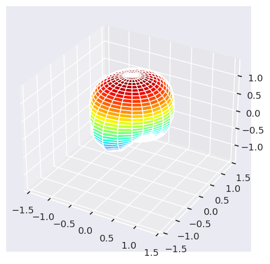
# The sum of these can be plotted directly... although may not be very useful
ep.sphSumPlotX(I)
*** WARNING: plot dataset has min value < 0, min = (-0.8400465549302628-0.43869471033269675j). This may be unphysical and/or result in plotting issues.
Sph plots:
Plotting with facetDims=Eke, pType=a with backend=mpl.
[4]:
[<Figure size 720x480 with 1 Axes>]
[5]:
# To plot components subselect on l first
# Set backend to Plotly for interactive panel plot
ep.sphSumPlotX(I.sel(l=2), facetDim = 'm', backend='pl');
*** WARNING: plot dataset has min value < 0, min = (-0.38607574059609784-9.456128398989102e-17j). This may be unphysical and/or result in plotting issues.
Sph plots:
Plotting with facetDims=m, pType=a with backend=pl.
*** Plotting for [1,1,0]
*** Plotting for [1,2,1]
*** Plotting for [1,3,2]
*** Plotting for [1,4,3]
*** Plotting for [1,5,4]
[6]:
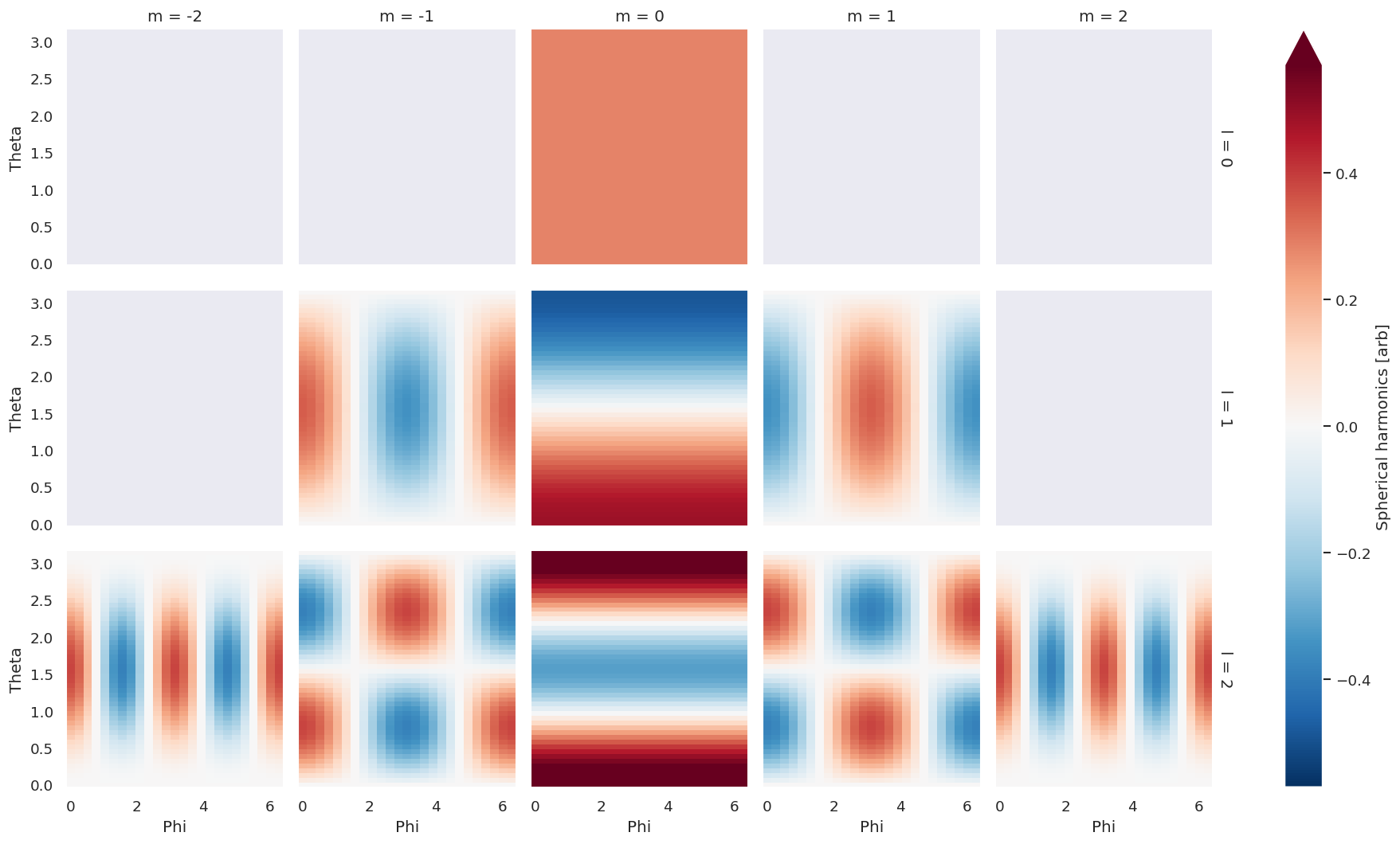
# Cart plots can be constructed directly with Xarray methods (NOTE this needs unstack() and .real or .imag)
I.real.unstack().plot(y='Theta', x='Phi', row='l', col='m', robust=True)
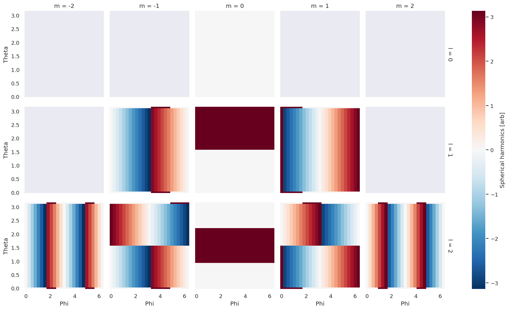
# For more data type options use ep.plotTypeSelector, e.g. plot phase
ep.plotTypeSelector(I.unstack('LM'), pType = 'phase').plot(y='Theta', x='Phi', row='l', col='m', robust=True)
[6]:
<xarray.plot.facetgrid.FacetGrid at 0x7fe4b5dfbe20>
[7]:
# Change plot style to default MPL
ep.basicPlotters.setPlotters(resetMpl=True)
* Set Holoviews with bokeh.
[8]:
# For Legendre Polynomials, set fnType = 'lg'
Ilg = ep.sphCalc(Lmax = 2, res = 50, fnType = 'lg')
ep.sphSumPlotX(Ilg)
Sph plots:
Plotting with facetDims=Eke, pType=a with backend=mpl.
[8]:
[<Figure size 640x480 with 1 Axes>]
[9]:
Ilg
[9]:
<xarray.DataArray 'PL' (LM: 9, Phi: 50, Theta: 50)>
1.0 1.0 1.0 1.0 1.0 1.0 1.0 ... 0.4225 0.2979 0.193 0.1096 0.04906 0.01231 0.0
Coordinates:
* LM (LM) object MultiIndex
* l (LM) int64 0 1 1 1 2 2 2 2 2
* m (LM) int64 0 -1 0 1 -2 -1 0 1 2
* Phi (Phi) float64 0.0 0.1282 0.2565 0.3847 ... 5.899 6.027 6.155 6.283
* Theta (Theta) float64 0.0 0.06411 0.1282 0.1923 ... 3.013 3.077 3.142
Attributes:
dataType: PL
long_name: Legendre polynomials
harmonics: {'dtype': 'Legendre polynomials', 'kind': 'complex', 'normTyp...
units: arbSetting coefficients
To manually set coefficients from lists or arrays, use the setBLMs() function.
[10]:
# Set specific LM coeffs by list with setBLMs, items are [l,m,value]
from epsproc.sphCalc import setBLMs
BLM = setBLMs([[0,0,1],[1,1,1],[2,2,1]]) # Note different index
BLM
[10]:
<xarray.DataArray 'BLM' (BLM: 3, t: 1)>
1 1 1
Coordinates:
* BLM (BLM) object MultiIndex
* l (BLM) int64 0 1 2
* m (BLM) int64 0 1 2
* t (t) int64 0
Attributes:
dataType: BLM
long_name: Beta parameters
units: arb
harmonics: {'dtype': 'Complex harmonics', 'kind': 'complex', 'normType':...[11]:
# Set specific LM coeffs by numpy array with setBLMs, items are [l,m,value]
from epsproc.sphCalc import setBLMs
BLM = setBLMs(np.array([[0,0,1],[1,1,1],[2,2,1]])) # Note different index
BLM
[11]:
<xarray.DataArray 'BLM' (BLM: 3, t: 1)>
1 1 1
Coordinates:
* BLM (BLM) object MultiIndex
* l (BLM) int64 0 1 2
* m (BLM) int64 0 1 2
* t (t) int64 0
Attributes:
dataType: BLM
long_name: Beta parameters
units: arb
harmonics: {'dtype': 'Complex harmonics', 'kind': 'complex', 'normType':...[12]:
# Set all allowed BLM up to Lmax with genLM
LM = ep.genLM(2)
# BLMall = setBLMs(np.ones([LM.shape[0],1]), LM)
BLMall = setBLMs(np.ones(LM.shape[0]), LM)
BLMall
[12]:
<xarray.DataArray 'BLM' (BLM: 9, t: 1)>
1.0 1.0 1.0 1.0 1.0 1.0 1.0 1.0 1.0
Coordinates:
* BLM (BLM) object MultiIndex
* l (BLM) int64 0 1 1 1 2 2 2 2 2
* m (BLM) int64 0 -1 0 1 -2 -1 0 1 2
* t (t) int64 0
Attributes:
dataType: BLM
long_name: Beta parameters
units: arb
harmonics: {'dtype': 'Complex harmonics', 'kind': 'complex', 'normType':...[13]:
# Set all allowed BLM up to Lmax with genLM, random value case
LM = ep.genLM(2)
BLMallrand = setBLMs(np.random.random(LM.shape[0]), LM)
BLMallrand
[13]:
<xarray.DataArray 'BLM' (BLM: 9, t: 1)>
0.494 0.44 0.2508 0.3413 0.629 0.1287 0.5041 0.7749 0.9317
Coordinates:
* BLM (BLM) object MultiIndex
* l (BLM) int64 0 1 1 1 2 2 2 2 2
* m (BLM) int64 0 -1 0 1 -2 -1 0 1 2
* t (t) int64 0
Attributes:
dataType: BLM
long_name: Beta parameters
units: arb
harmonics: {'dtype': 'Complex harmonics', 'kind': 'complex', 'normType':...Note that the function adds a t dimension, which is used as a generic index in these cases. For 1D cases it can be dropped by squeezing the array:
[14]:
BLMallrand = BLMallrand.squeeze(drop=True)
BLMallrand
[14]:
<xarray.DataArray 'BLM' (BLM: 9)>
0.494 0.44 0.2508 0.3413 0.629 0.1287 0.5041 0.7749 0.9317
Coordinates:
* BLM (BLM) object MultiIndex
* l (BLM) int64 0 1 1 1 2 2 2 2 2
* m (BLM) int64 0 -1 0 1 -2 -1 0 1 2
Attributes:
dataType: BLM
long_name: Beta parameters
units: arb
harmonics: {'dtype': 'Complex harmonics', 'kind': 'complex', 'normType':...… or, for cases \(\beta_{L,M}(t)\), can be set directly (or renamed and used for other coords). Currently only a single dimension is supported here.
[15]:
# Set all allowed BLM up to Lmax with genLM, random value case, and as a function of t
# If coordinates are not specified, integer labels are used.
LM = ep.genLM(2)
BLMallrandt = setBLMs(np.random.random([LM.shape[0],5]), LM)
BLMallrandt
[15]:
<xarray.DataArray 'BLM' (BLM: 9, t: 5)>
0.2849 0.8737 0.4825 0.7058 0.6063 ... 0.8563 0.5342 0.3983 0.8242 0.5575
Coordinates:
* BLM (BLM) object MultiIndex
* l (BLM) int64 0 1 1 1 2 2 2 2 2
* m (BLM) int64 0 -1 0 1 -2 -1 0 1 2
* t (t) int64 0 1 2 3 4
Attributes:
dataType: BLM
long_name: Beta parameters
units: arb
harmonics: {'dtype': 'Complex harmonics', 'kind': 'complex', 'normType':...For a tabulation of the expansion parameters (via Pandas), use tabulateLM.
[16]:
from epsproc.sphFuncs.sphConv import tabulateLM
tabulateLM(BLMallrand)
[16]:
| m | -2 | -1 | 0 | 1 | 2 |
|---|---|---|---|---|---|
| l | |||||
| 0 | 0.000000 | 0.000000 | 0.494049 | 0.000000 | 0.000000 |
| 1 | 0.000000 | 0.439969 | 0.250776 | 0.341302 | 0.000000 |
| 2 | 0.628958 | 0.128726 | 0.504075 | 0.774880 | 0.931717 |
Calculating & plotting expansions
This can be done manually with Xarray multiplications for full control, or via the function sphFromBLMPlot(). Note this will use self.attrs['harmonics'] from the input data to define the harmonics used, or default to complex harmonics if not specified.
(Note that some higher-level plotting routines are provided in the base class.)
[17]:
# Direct Xarray tensor multiplication - this will correctly handle dimensions if names match.
Irand = BLMallrand.rename({'BLM':'LM'}) * Isph
# ep.sphSumPlotX(Irand, facetDim = 't') # Note this may need facetDim set explicitly here for non-1D cases
ep.sphSumPlotX(Irand)
Irand
*** WARNING: plot dataset has min value < 0, min = (-0.6224372110620724-0.2398106684194127j). This may be unphysical and/or result in plotting issues.
Sph plots:
Plotting with facetDims=Eke, pType=a with backend=mpl.
[17]:
<xarray.DataArray (LM: 9, Phi: 50, Theta: 50)> (0.13936862703536948+0j) (0.13936862703536948+0j) ... 0j Coordinates: * LM (LM) object MultiIndex * l (LM) int64 0 1 1 1 2 2 2 2 2 * m (LM) int64 0 -1 0 1 -2 -1 0 1 2 * Phi (Phi) float64 0.0 0.1282 0.2565 0.3847 ... 5.899 6.027 6.155 6.283 * Theta (Theta) float64 0.0 0.06411 0.1282 0.1923 ... 3.013 3.077 3.142

[18]:
# Functional form - this returns array, include plotFlag = True to show plot and return a fig handle
# Note this will use `BLM.attrs['harmonics']` to define the harmonics used, or default to complex harmonics if not specified.
Itp, fig = ep.sphFromBLMPlot(BLMallrand, plotFlag = True)
Itp
Using complex betas (from BLMX array).
*** WARNING: plot dataset has min value < 0, min = (-0.6224372110620724-0.2398106684194127j). This may be unphysical and/or result in plotting issues.
Sph plots:
Plotting with facetDims=None, pType=a with backend=mpl.
[18]:
<xarray.DataArray (LM: 9, Phi: 50, Theta: 50)>
(0.13936862703536948+0j) (0.13936862703536948+0j) ... 0j
Coordinates:
* LM (LM) object MultiIndex
* l (LM) int64 0 1 1 1 2 2 2 2 2
* m (LM) int64 0 -1 0 1 -2 -1 0 1 2
* Phi (Phi) float64 0.0 0.1282 0.2565 0.3847 ... 5.899 6.027 6.155 6.283
* Theta (Theta) float64 0.0 0.06411 0.1282 0.1923 ... 3.013 3.077 3.142
Attributes:
dataType: Itp
long_name: I(\theta,\phi)
harmonics: {'dtype': 'Complex harmonics', 'kind': 'complex', 'normType':...
units: arb
normType: complex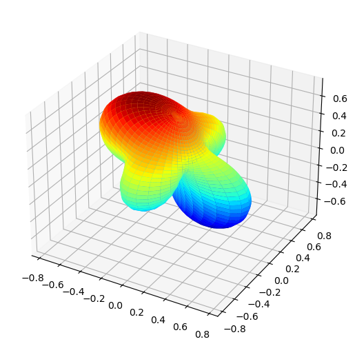
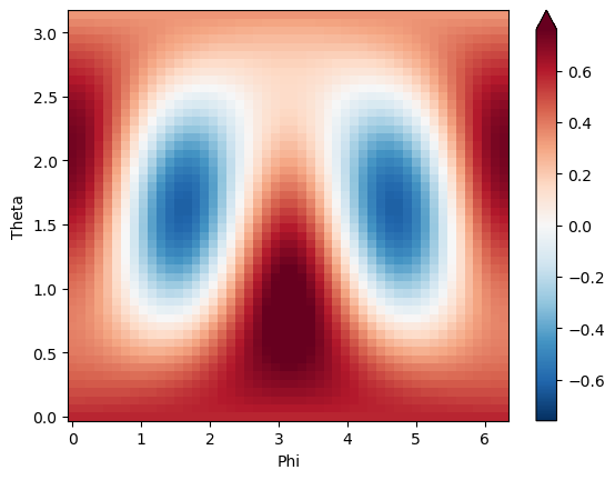
[19]:
# For a Cartesian plot, this can be done directly with Xarray functionality
# Note some dim handling may be required here.
# Plot sum, real part
Itp.sum('LM').real.plot(y='Theta',x='Phi', robust=True)
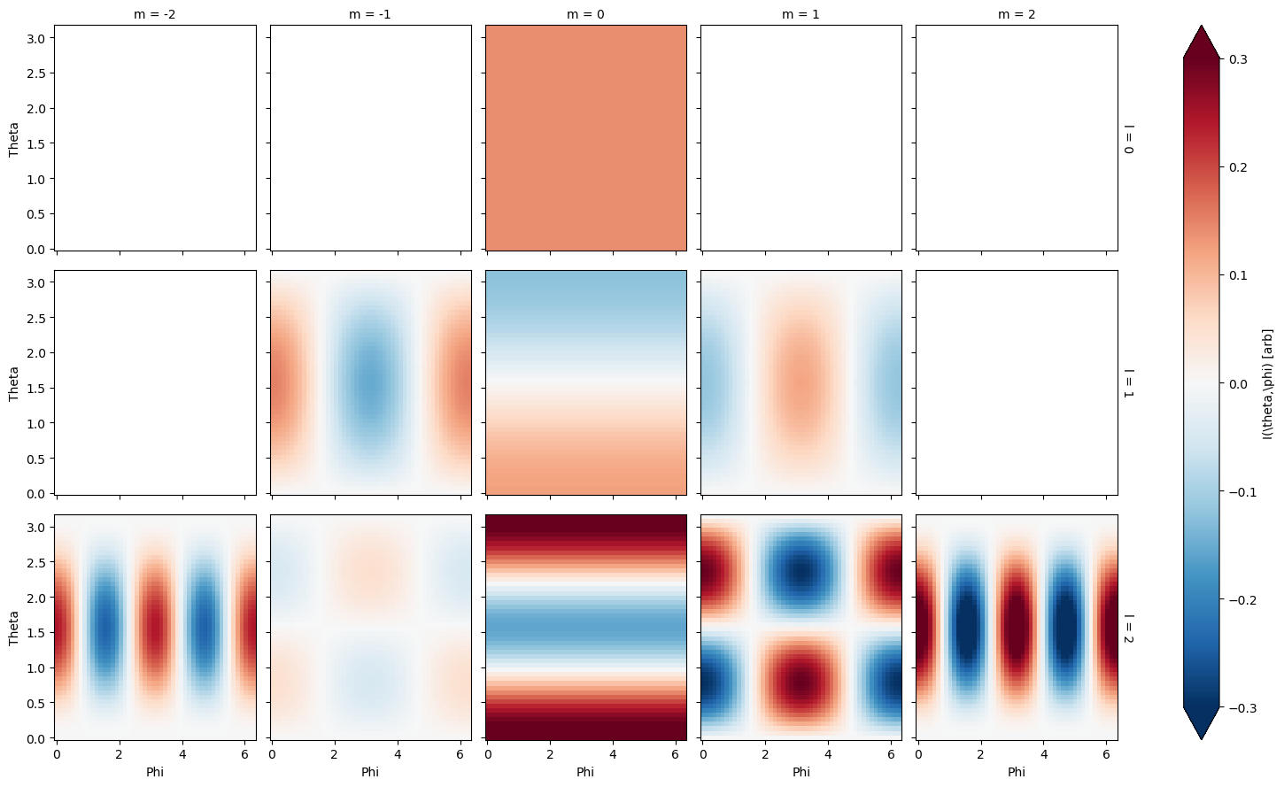
# Plot components, abs values
# Itp.unstack('LM').pipe(np.abs).plot(y='Theta', x='Phi', row='l', col='m', robust=True)
# Plot components, real values
Itp.unstack('LM').real.plot(y='Theta', x='Phi', row='l', col='m', robust=True)
[19]:
<xarray.plot.facetgrid.FacetGrid at 0x7fe59cc31970>
[20]:
# Set the backend to 'pl' for an interactive surface plot with Plotly
ep.sphFromBLMPlot(BLMallrandt, facetDim = 't', plotFlag = True, backend = 'pl');
Using complex betas (from BLMX array).
*** WARNING: plot dataset has min value < 0, min = (-0.582750353156348-0.30737321609288326j). This may be unphysical and/or result in plotting issues.
Sph plots:
Plotting with facetDims=t, pType=a with backend=pl.
*** Plotting for [1,1,0]
*** Plotting for [1,2,1]
*** Plotting for [1,3,2]
*** Plotting for [1,4,3]
*** Plotting for [1,5,4]
Conversions
Coefficient conversion
To convert \(\beta_{L,M}\) normalisations and types, a few utility functions are implemented.
[21]:
# Set some terms - note the BLM values are initially unlabelled by normType or with 'harmonics' attribututes.
LM = ep.genLM(Lmax =2, allM=False)
Blg = setBLMs(np.random.random(LM.shape[0]), LM, dtype = 'Lg', kind = 'real') # Additional labels are set in Blg.attrs['harmonics']
#.sel(m=0, drop=False) # Testing in XR 2022.3.0, this ALWAYS drops m for stacked dim case - should add some dim handling to conv_BL_BLM()!
Blg
[21]:
<xarray.DataArray 'BLM' (BLM: 3, t: 1)>
0.7223 0.4495 0.19
Coordinates:
* BLM (BLM) object MultiIndex
* l (BLM) int64 0 1 2
* m (BLM) int64 0 0 0
* t (t) int64 0
Attributes:
dataType: BLM
long_name: Beta parameters
units: arb
harmonics: {'dtype': 'Lg', 'kind': 'real', 'normType': 'ortho', 'csPhase...[22]:
# Convert from Sph to Lg normalised values and don't renormalise
Bsp = ep.util.conversion.conv_BL_BLM(Blg, to='sph', renorm=False)
Bsp
[22]:
<xarray.DataArray (BLM: 3, t: 1)>
2.561 0.9199 0.3012
Coordinates:
* BLM (BLM) object MultiIndex
* l (BLM) int64 0 1 2
* m (BLM) int64 0 0 0
* t (t) int64 0
Attributes:
dataType: BLM
long_name: Beta parameters
units: arb
harmonics: {'dtype': 'sph', 'kind': 'real', 'normType': 'ortho', 'csPhas...
normType: sphGenerating conjugate terms
[23]:
LM = ep.genLM(Lmax =2)
Bpos = setBLMs(np.random.random(LM.shape[0]), LM)
Bpos = Bpos.where(Bpos.m > -1, drop=True) # Select m=0 or +ve only
Bpos
[23]:
<xarray.DataArray 'BLM' (BLM: 6, t: 1)>
0.7004 0.4311 0.8393 0.4666 0.02414 0.8502
Coordinates:
* BLM (BLM) object MultiIndex
* l (BLM) int64 0 1 1 2 2 2
* m (BLM) int64 0 0 1 0 1 2
* t (t) int64 0
Attributes:
dataType: BLM
long_name: Beta parameters
units: arb
harmonics: {'dtype': 'Complex harmonics', 'kind': 'complex', 'normType':...[24]:
# Get complex conjugate terms (for -m)
from epsproc.sphFuncs.sphConv import sphConj
sphConj(Bpos)
[24]:
<xarray.DataArray (t: 1, BLM: 6)>
0.7004 0.4311 -0.8393 0.4666 -0.02414 0.8502
Coordinates:
* t (t) int64 0
* BLM (BLM) object MultiIndex
* l (BLM) int64 0 1 1 2 2 2
* m (BLM) int64 0 0 -1 0 -1 -2
Attributes:
dataType: BLM
long_name: Beta parameters
units: arb
harmonics: {'dtype': 'Complex harmonics', 'kind': 'complex', 'normType':...SHtools conversion
To convert values to SHtools objects, use epsproc.sphFuncs.sphConv.SHcoeffsFromXR(). Note this currently (Sept. 2022) only supports 1D input arrays.
For a list of SHtools object methods, see the SHtools ‘SHCoeffs’ class docs.
[25]:
BLMallrand
[25]:
<xarray.DataArray 'BLM' (BLM: 9)>
0.494 0.44 0.2508 0.3413 0.629 0.1287 0.5041 0.7749 0.9317
Coordinates:
* BLM (BLM) object MultiIndex
* l (BLM) int64 0 1 1 1 2 2 2 2 2
* m (BLM) int64 0 -1 0 1 -2 -1 0 1 2
Attributes:
dataType: BLM
long_name: Beta parameters
units: arb
harmonics: {'dtype': 'Complex harmonics', 'kind': 'complex', 'normType':...[26]:
from epsproc.sphFuncs.sphConv import *
# Create SHtools object - this will use settings in data.attrs['harmonics'], or passed args
sh = SHcoeffsFromXR(BLMallrand) #, kind = 'real'
sh
[26]:
kind = 'complex'
normalization = 'ortho'
csphase = 1
lmax = 2
error_kind = None
header = None
header2 = None
name = None
units = None
[27]:
# Check parameters - this are set as a 3D array, where the SHtools convention is to index as [+/-,l,m]
sh.coeffs
[27]:
array([[[0.49404892+0.j, 0. +0.j, 0. +0.j],
[0.25077562+0.j, 0.34130211+0.j, 0. +0.j],
[0.5040749 +0.j, 0.77487963+0.j, 0.93171739+0.j]],
[[0. +0.j, 0. +0.j, 0. +0.j],
[0. +0.j, 0.4399693 +0.j, 0. +0.j],
[0. +0.j, 0.12872607+0.j, 0.62895844+0.j]]])
[28]:
# SHtools has various conversion and util routines, see https://shtools.github.io/SHTOOLS/python-shcoeffs.html
sh4p = sh.convert(csphase =1 , normalization='4pi')
sh4p
[28]:
kind = 'complex'
normalization = '4pi'
csphase = 1
lmax = 2
error_kind = None
header = None
header2 = None
name = None
units = None
[29]:
sh4p.coeffs
[29]:
array([[[0.13936863+0.j, 0. +0.j, 0. +0.j],
[0.0707425 +0.j, 0.09627955+0.j, 0. +0.j],
[0.1421969 +0.j, 0.21858951+0.j, 0.26283262+0.j]],
[[0. +0.j, 0. +0.j, 0. +0.j],
[0. +0.j, 0.12411305+0.j, 0. +0.j],
[0. +0.j, 0.03631295+0.j, 0.1774259 +0.j]]])
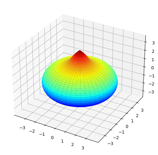
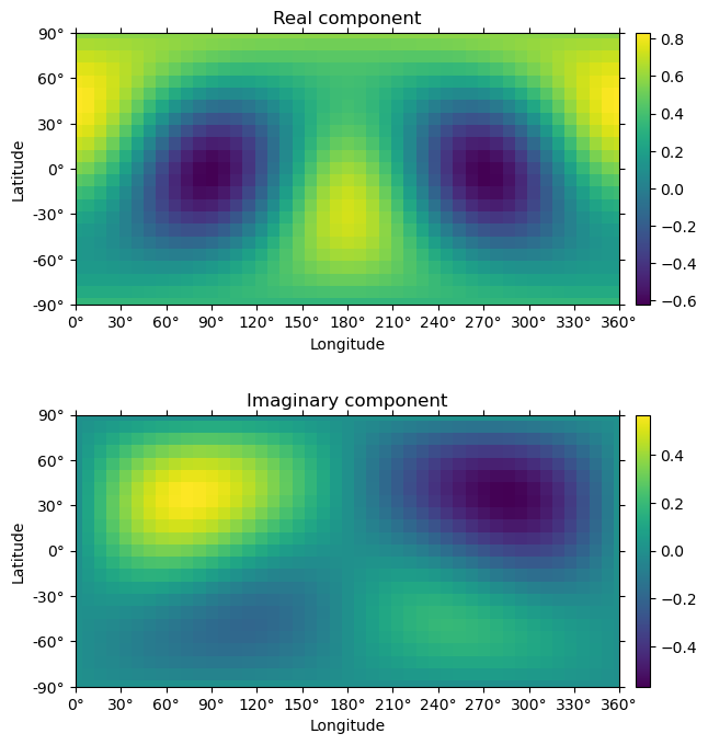
[30]:
# SHtools expand on grid & plot
lmaxGrid = 10
grid = sh.expand(lmax = lmaxGrid)
grid.plot(colorbar='right')
[30]:
(<Figure size 640x704 with 4 Axes>,
array([<AxesSubplot:title={'center':'Real component'}, xlabel='Longitude', ylabel='Latitude'>,
<AxesSubplot:title={'center':'Imaginary component'}, xlabel='Longitude', ylabel='Latitude'>],
dtype=object))
[31]:
# Convert SHtools object to Xarray
# This converts coords to (l,m) index, and SHtools object to to .attrs['SH']
shXR = XRcoeffsFromSH(sh)
shXR
[31]:
<xarray.DataArray (LM: 9)>
(0.4940489193685105+0j) (0.2507756219705549+0j) ... (0.6289584448927145+0j)
Coordinates:
* LM (LM) object MultiIndex
* l (LM) int64 0 1 1 1 2 2 2 2 2
* m (LM) int64 0 0 1 -1 0 1 2 -1 -2
Attributes:
SH: kind = 'complex'\nnormalization = 'ortho'\ncsphase = 1\nlmax ...
harmonics: {'dtype': 'Harmonics from SHtools', 'kind': 'complex', 'normT...Versions
[32]:
import scooby
scooby.Report(additional=['epsproc', 'holoviews', 'hvplot', 'xarray', 'matplotlib', 'bokeh'])
[32]:
| Wed Sep 28 18:55:07 2022 UTC | |||||||
| OS | Linux | CPU(s) | 32 | Machine | x86_64 | Architecture | 64bit |
| RAM | 50.1 GiB | Environment | Jupyter | ||||
| Python 3.9.10 | packaged by conda-forge | (main, Feb 1 2022, 21:24:11) [GCC 9.4.0] | |||||||
| epsproc | 1.3.2-dev | holoviews | 1.14.8 | hvplot | Module not found | xarray | 2022.6.0 |
| matplotlib | 3.5.1 | bokeh | 2.4.2 | numpy | 1.21.5 | scipy | 1.8.0 |
| IPython | 8.1.1 | scooby | 0.5.12 | ||||
[33]:
# Check current Git commit for local ePSproc version
from pathlib import Path
!git -C {Path(ep.__file__).parent} branch
!git -C {Path(ep.__file__).parent} log --format="%H" -n 1
* dev
master
numba-tests
0a15eb6cf4e469446efbf0ab2518d3fb1e64dfdb
[34]:
# Check current remote commits
!git ls-remote --heads https://github.com/phockett/ePSproc
92c661789a7d2927f2b53d7266f57de70b3834fa refs/heads/dependabot/pip/notes/envs/envs-versioned/mistune-2.0.3
fe1e9540c7b91fe571f60562acd31d8e489d491e refs/heads/dependabot/pip/notes/envs/envs-versioned/nbconvert-6.5.1
0a15eb6cf4e469446efbf0ab2518d3fb1e64dfdb refs/heads/dev
1c0b8fd409648f07c85f4f20628b5ea7627e0c4e refs/heads/master
69cd89ce5bc0ad6d465a4bd8df6fba15d3fd1aee refs/heads/numba-tests
ea30878c842f09d525fbf39fa269fa2302a13b57 refs/heads/revert-9-master