ePSproc base and multijob class intro
16/10/20
As of Oct. 2020, v1.3.0-dev, basic data classes are now implemented, and are now the easiest/preferred method for using ePSproc (as opposed to calling core functions directly, as illustrated in the functions guide).
A brief intro and guide to use is given here.
Aims:
Provide unified data architecture for ePSproc, ePSdata and PEMtk.
Wrap plotting and computational functions for ease of use.
Handle multiple datasets inc. comparitive plots.
Setup
[1]:
# For module testing, include path to module here, otherwise use global installation
local = True
if local:
import sys
if sys.platform == "win32":
modPath = r'D:\code\github\ePSproc' # Win test machine
winFlag = True
else:
modPath = r'/home/femtolab/github/ePSproc/' # Linux test machine
winFlag = False
sys.path.append(modPath)
# Base
import epsproc as ep
# Class dev code
from epsproc.classes.multiJob import ePSmultiJob
from epsproc.classes.base import ePSbase
* pyevtk not found, VTK export not available.
ePSbase class
The ePSbase class wraps most of the core functionality, and will handle all ePolyScat output files in a single data directory. In general, we’ll assume:
an ePS job constitutes a single ionization event/channel (ionizing orbital) for a given molecule, stored in one or more output files.
the data dir contains one or more files, where each file will contain a set of symmetries and energies, with either
one file per ionizing event. In this case, each file will equate to one job, and one entry in the class datastructure.
a single ionizing event, where each file contains a different set of energies for the given event (energy chunked fileset). In this case, the files will be stacked, and the dir will equate to one job and one entry in the class datastructure.
The class datastructure is (currently) a set of dictionaries, with entries per job as above, and various data for each job. In general the data is stored in Xarrays.
The multiJob class extends the base class with reading from multple directories.
Load data
Firstly, set the data path, instantiate a class object and load the data.
[2]:
# Set for ePSproc test data, available from https://github.com/phockett/ePSproc/tree/master/data
# Here this is assumed to be on the epsproc path
import os
dataPath = os.path.join(sys.path[-1], 'data', 'photoionization', 'n2_multiorb')
[3]:
# Instantiate class object.
# Minimally this needs just the dataPath, if verbose = 1 is set then some useful output will also be printed.
data = ePSbase(dataPath, verbose = 1)
[4]:
# ScanFiles() - this will look for data files on the path provided, and read from them.
data.scanFiles()
*** Job orb6 details
Key: orb6
Dir D:\code\github\ePSproc\data\photoionization\n2_multiorb, 1 files.
{ 'batch': 'ePS n2, batch n2_1pu_0.1-50.1eV, orbital A2',
'event': ' N2 A-state (1piu-1)',
'orbE': -17.096913836366,
'orbLabel': '1piu-1'}
*** Job orb5 details
Key: orb5
Dir D:\code\github\ePSproc\data\photoionization\n2_multiorb, 1 files.
{ 'batch': 'ePS n2, batch n2_3sg_0.1-50.1eV, orbital A2',
'event': ' N2 X-state (3sg-1)',
'orbE': -17.341816310545997,
'orbLabel': '3sg-1'}
In this case, two files are read, and each file is a different ePS job - here the \(3\sigma_g^{-1}\) and \(1\pi_u^{-1}\) channels in N2. The keys for the job are also used as the job names.
Basic info & plots
A few basic methods to summarise the data…
[5]:
# Summarise jobs, this will also be output by scanFile() if verbose = 1 is set, as illustrated above.
data.jobsSummary()
*** Job orb6 details
Key: orb6
Dir D:\code\github\ePSproc\data\photoionization\n2_multiorb, 1 files.
{ 'batch': 'ePS n2, batch n2_1pu_0.1-50.1eV, orbital A2',
'event': ' N2 A-state (1piu-1)',
'orbE': -17.096913836366,
'orbLabel': '1piu-1'}
*** Job orb5 details
Key: orb5
Dir D:\code\github\ePSproc\data\photoionization\n2_multiorb, 1 files.
{ 'batch': 'ePS n2, batch n2_3sg_0.1-50.1eV, orbital A2',
'event': ' N2 X-state (3sg-1)',
'orbE': -17.341816310545997,
'orbLabel': '3sg-1'}
[6]:
# Molecular info
# Note that this is currently assumed to be the same for all jobs in the data dir.
data.molSummary()
*** Molecular structure
*** Molecular orbital list (from ePS output file)
EH = Energy (Hartrees), E = Energy (eV), NOrbGrp, OrbGrp, GrpDegen = degeneracies and corresponding orbital numbering by group in ePS, NormInt = single centre expansion convergence (should be ~1.0).
| props | Sym | EH | Occ | E | NOrbGrp | OrbGrp | GrpDegen | NormInt |
|---|---|---|---|---|---|---|---|---|
| orb | ||||||||
| 1 | SG | -15.6719 | 2.0 | -426.454121 | 1.0 | 1.0 | 1.0 | 0.999532 |
| 2 | SU | -15.6676 | 2.0 | -426.337112 | 1.0 | 2.0 | 1.0 | 0.999458 |
| 3 | SG | -1.4948 | 2.0 | -40.675580 | 1.0 | 3.0 | 1.0 | 0.999979 |
| 4 | SU | -0.7687 | 2.0 | -20.917392 | 1.0 | 4.0 | 1.0 | 0.999979 |
| 5 | SG | -0.6373 | 2.0 | -17.341816 | 1.0 | 5.0 | 1.0 | 1.000000 |
| 6 | PU | -0.6283 | 2.0 | -17.096914 | 1.0 | 6.0 | 2.0 | 1.000000 |
| 7 | PU | -0.6283 | 2.0 | -17.096914 | 2.0 | 6.0 | 2.0 | 1.000000 |
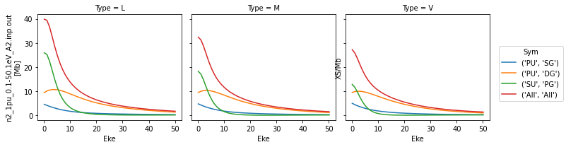
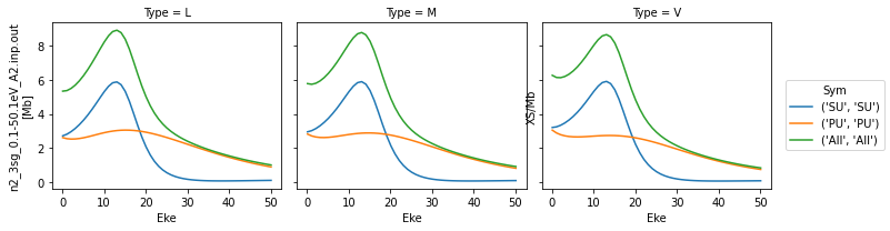
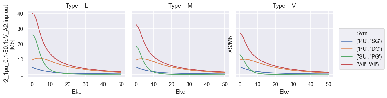
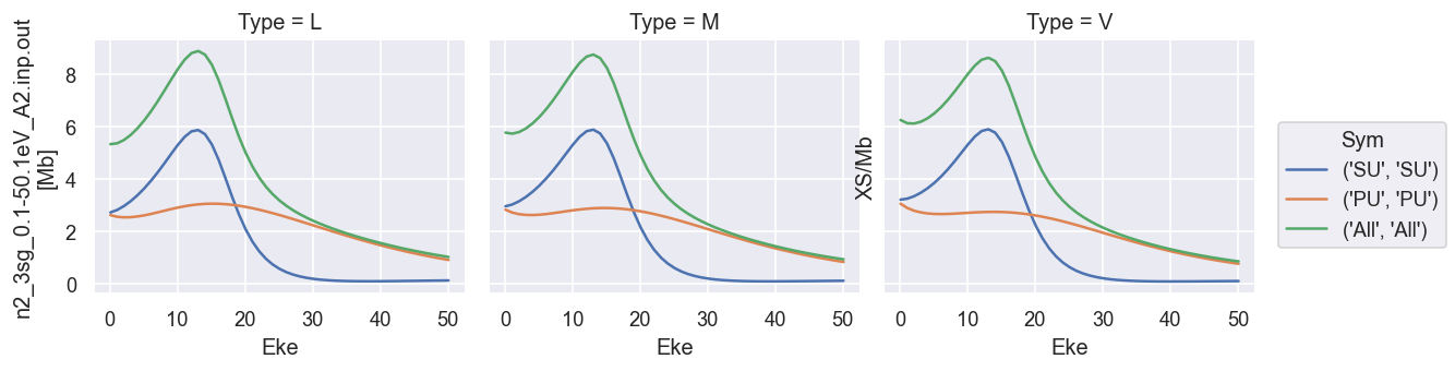
Plot cross-sections and betas
These are taken from the GetCro segments in the ePS output files, and correspond to results for an isotropic ensemble of molecules, i.e. observables in the lab frame (LF) for 1-photon ionization (see the ePS tutorial for more details).
[7]:
# Minimal method call will plot cross-sections for all ePS jobs found in the data directory.
data.plotGetCro()
[8]:
# Plot beta parameters with the 'BETA' flag
data.plotGetCro(pType = 'BETA')
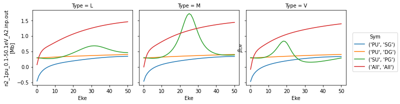
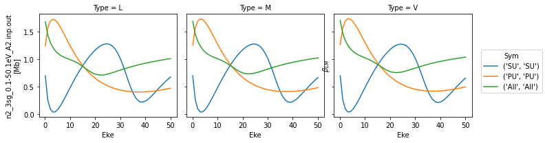
TODO: fix labelling here.
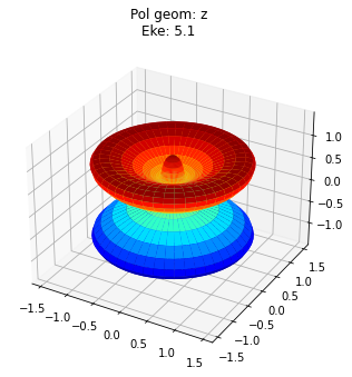
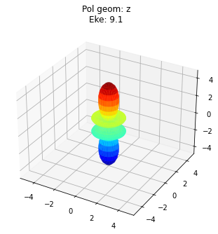
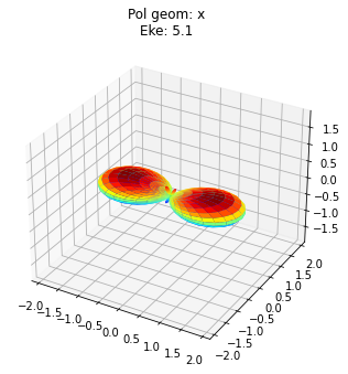
Compute MFPADs
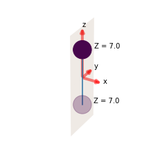
The class currently wraps just the basic numerical routine for MFPADs. This defaults to computing MFPADs for all energies and \((z,x,y)\) polarization geometries (where the z-axis is the molecular symmetry axis, and corresponds to the molecular structure plot shown above).
[9]:
# Compute MFPADs...
data.mfpadNumeric()
To plot it’s advisable to set an enery slice, Erange = [start, stop, step], since MFPADs are currently shown as individual plots in the default case, and there may be a lot of them.
We’ll also just set for a single key here, otherwise all jobs will be plotted.
[10]:
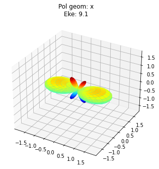
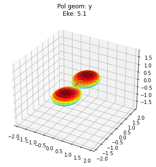
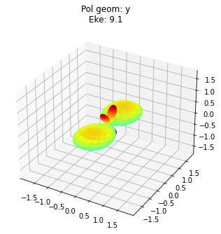
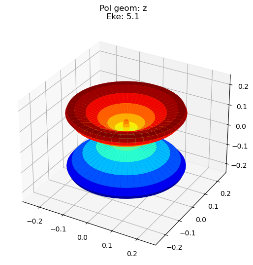
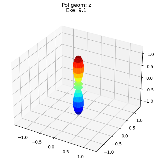
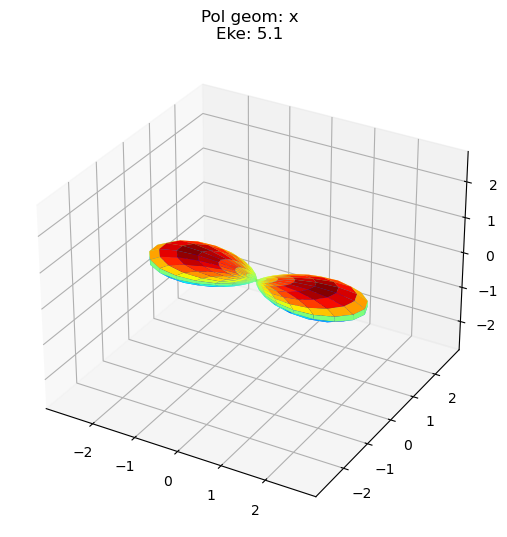
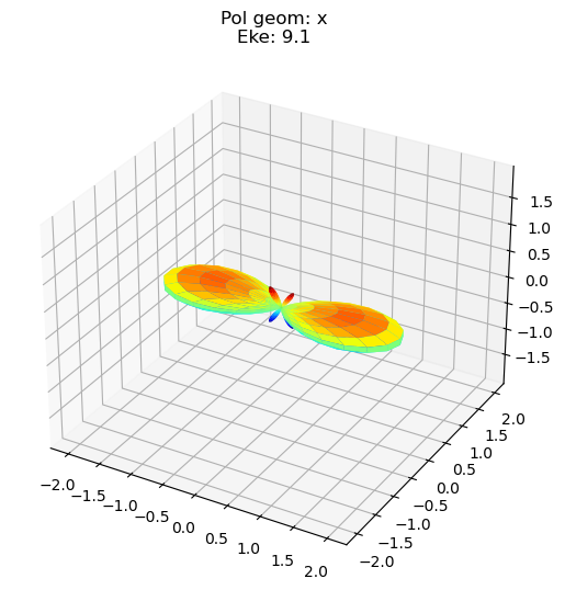
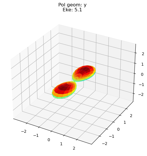
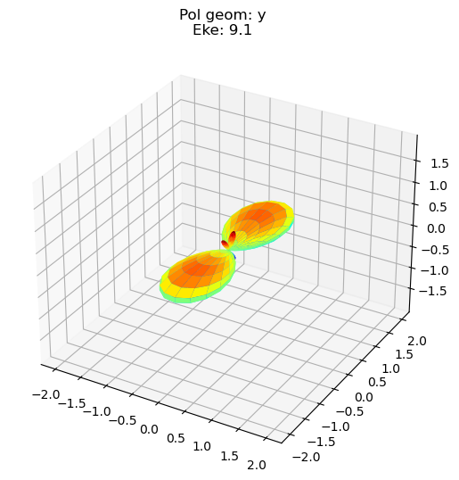
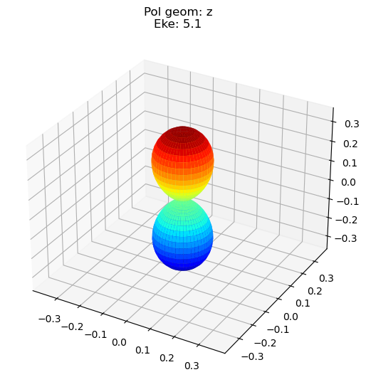
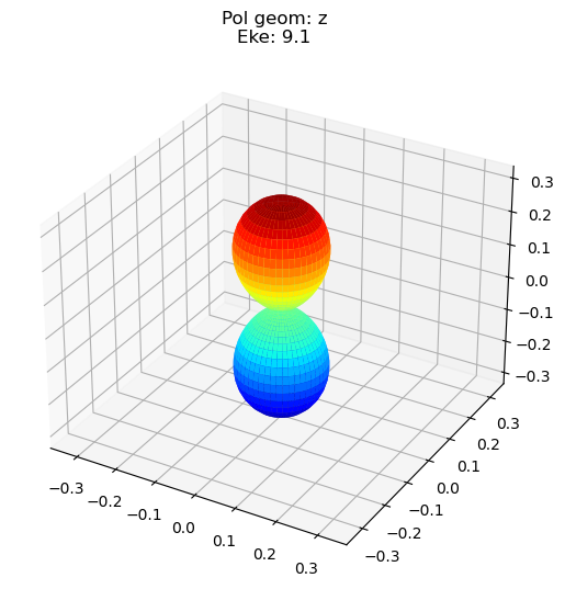
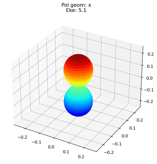
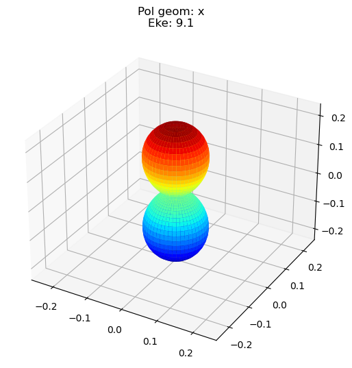
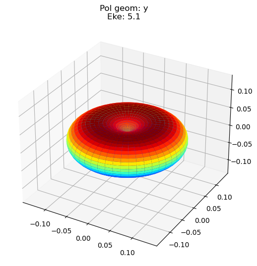
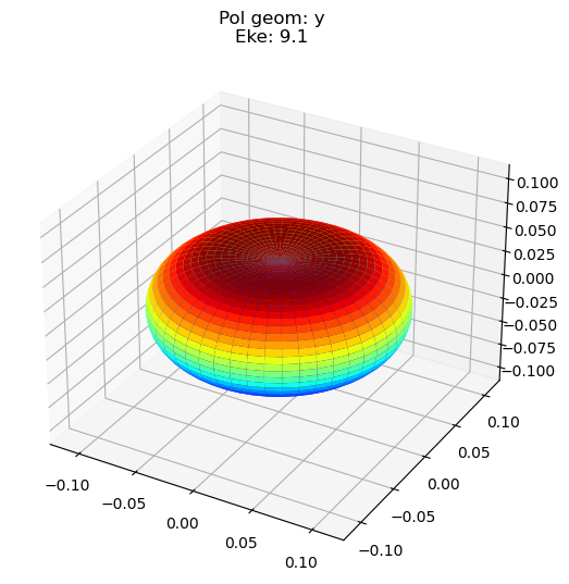
data.padPlot(keys = 'orb5', Erange = [5, 10, 4])
#TODO: fix plot layout!
Found dims ('Labels', 'Phi', 'Theta', 'Eke', 'Sym'), summing to reduce for plot. Pass selDims to avoid.
Sph plots: Pol geom: z
Plotting with mpl
Data dims: ('Phi', 'Theta', 'Eke'), subplots on Eke
Sph plots: Pol geom: x
Plotting with mpl
Data dims: ('Phi', 'Theta', 'Eke'), subplots on Eke
Sph plots: Pol geom: y
Plotting with mpl
Data dims: ('Phi', 'Theta', 'Eke'), subplots on Eke
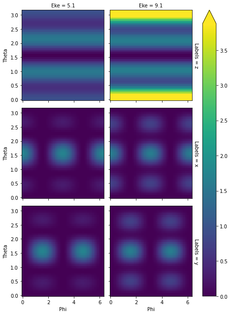
To view multiple results in a more concise fashion, a Cartesian gridded output is also available.
[11]:
data.padPlot(keys = 'orb5', Erange = [5, 10, 4], pStyle='grid')
Found dims ('Labels', 'Phi', 'Theta', 'Eke', 'Sym'), summing to reduce for plot. Pass selDims to avoid.
Grid plot: 3sg-1
[12]:
# Various other args can be passed...
# Set a plotting backend, currently 'mpl' (Matplotlib - default) or 'pl' (Plotly - interactive, but may give issues in some environments)
backend = 'pl'
# Subselect on dimensions, this is set as a dictionary for Xarray selection (see http://xarray.pydata.org/en/stable/indexing.html#indexing-with-dimension-names)
selDims = {'Labels':'z'} # Plot z-pol case only.
data.padPlot(Erange = [5, 10, 4], selDims=selDims, backend = backend)
Found dims ('Phi', 'Theta', 'Eke', 'Sym'), summing to reduce for plot. Pass selDims to avoid.
Sph plots: 1piu-1
Plotting with pl
Found dims ('Phi', 'Theta', 'Eke', 'Sym'), summing to reduce for plot. Pass selDims to avoid.
Sph plots: 3sg-1
Plotting with pl
Compute \(\beta_{LM}\) parameters
For computation of \(\beta_{LM}\) parameters the class wraps functions from epsproc.geom, which implement a tensor method. This is quite fast, although memory heavy, so may not be suitable for very large problems. (See the method development pages for more info, more concise notes to follow).
Functions are provided for MF and AF problems (which is the general case, and will equate to the LF case for an unaligned ensemble).
For the MF the class wraps
ep.geom.mfblmXprod, see the method development page for more info, more concise notes to follow.For the AF the class wraps
ep.geom.afblmXprod, see the method development page for more info, more concise notes to follow.
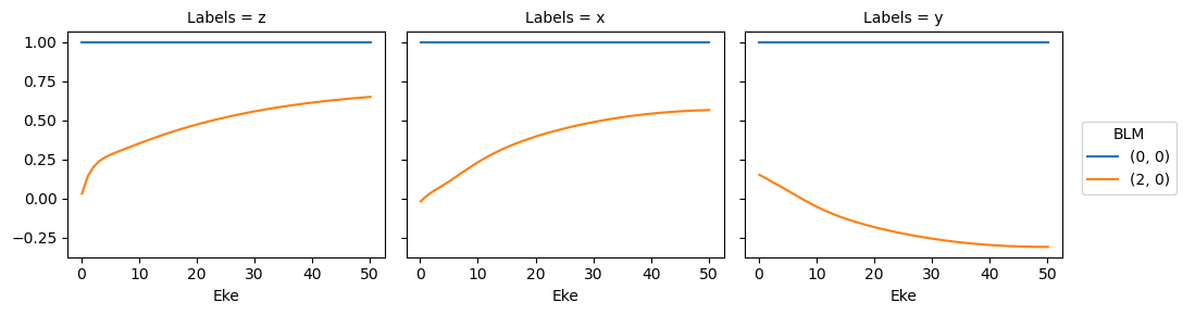
Compute MF \(\beta_{LM}\) and PADs
Here’s a quick demo for the default MF cases, which will give parameters corresponding to the \((z,x,y)\) polarization geometries computed by the numerical routine above.
[13]:
data.MFBLM()
Calculating MF-BLMs for job key: orb6
Return type BLM.
Calculating MF-BLMs for job key: orb5
Return type BLM.
Plotting still needs to improve… but ep.lmPlot() is a robust way to plot everything.
[14]:
# data.BLMplot(dataType = 'MFBLM') # HORRIBLE OUTPUT at the moment!!!
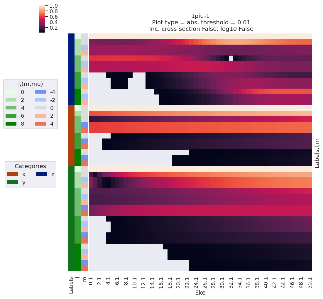
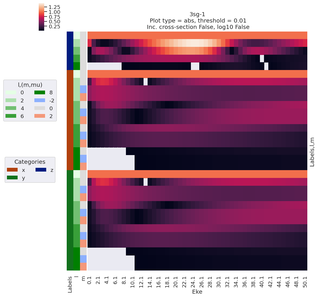
data.lmPlot(dataType = 'MFBLM')
Plotting data n2_1pu_0.1-50.1eV_A2.inp.out, pType=a, thres=0.01, with Seaborn
Plotting data n2_3sg_0.1-50.1eV_A2.inp.out, pType=a, thres=0.01, with Seaborn
Line-plots are available with the BLMplot method, although this currently only supports the Matplotlib backend, and may have problems with dims in some cases (work in progress!).
[15]:
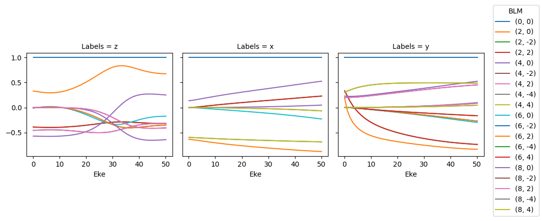
data.BLMplot(dataType='MFBLM', thres = 1e-2) # Passing a threshold value here will remove any spurious BLM parameters.
Dataset: orb6, 1piu-1, MFBLM
Dataset: orb5, 3sg-1, MFBLM
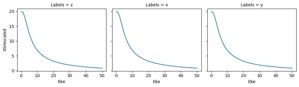
Polar plots are available for these distributions using the padPlot() method if the dataType is passed.
[16]:
data.padPlot(keys = 'orb5', Erange = [5, 10, 4], dataType='MFBLM')
Using default sph betas.
Sph plots: Pol geom: z
Plotting with mpl
Data dims: ('Eke', 'Phi', 'Theta'), subplots on Eke
Sph plots: Pol geom: x
Plotting with mpl
Data dims: ('Eke', 'Phi', 'Theta'), subplots on Eke
Sph plots: Pol geom: y
Plotting with mpl
Data dims: ('Eke', 'Phi', 'Theta'), subplots on Eke
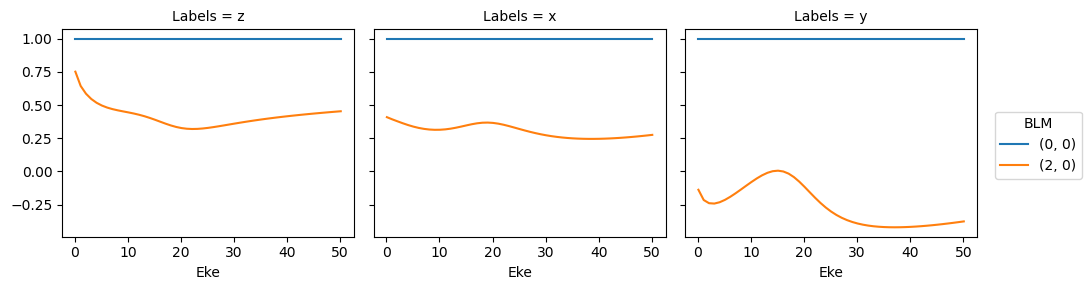
Compute LF/AF \(\beta_{LM}\) and PADs
Here’s a quick demo for the default AF case (isotropic distribution, hence == LF case).
[17]:
data.AFBLM()
Calculating AF-BLMs for job key: orb6
Calculating AF-BLMs for job key: orb5
Plotting still needs to improve… but ep.lmPlot() is a robust way to plot everything.
[18]:
# data.BLMplot(dataType = 'MFBLM') # HORRIBLE OUTPUT at the moment!!!
data.lmPlot(dataType = 'AFBLM')
Plotting data n2_1pu_0.1-50.1eV_A2.inp.out, pType=a, thres=0.01, with Seaborn
Plotting data n2_3sg_0.1-50.1eV_A2.inp.out, pType=a, thres=0.01, with Seaborn
Line-plots are available with the BLMplot method, although this currently only supports the Matplotlib backend, and may have problems with dims in some cases (work in progress!).
[19]:
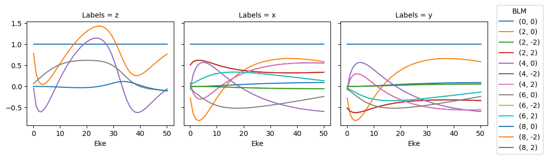
data.BLMplot(dataType='AFBLM', thres = 1e-2) # Passing a threshold value here will remove any spurious BLM parameters.
Dataset: orb6, 1piu-1, XS
Dataset: orb6, 1piu-1, AFBLM
Dataset: orb5, 3sg-1, XS
Dataset: orb5, 3sg-1, AFBLM
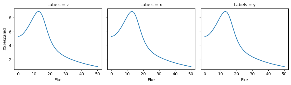
Polar plots are available for these distributions using the padPlot() method.
[20]:
data.padPlot(keys = 'orb5', Erange = [5, 10, 4], dataType='AFBLM')
# NOTE - seem to have an inconsistency with (x,y) pol geometries here - should check source code & fix. Likely due to mix-up in frame defns., i.e. probably mixing LF and MF pol geom defn. - TBC.
Found dims ('Labels', 't', 'Eke', 'BLM'), summing to reduce for plot. Pass selDims to avoid.
Using default sph betas.
Sph plots: Pol geom: z
Plotting with mpl
Data dims: ('t', 'Eke', 'Phi', 'Theta'), subplots on Eke
Sph plots: Pol geom: x
Plotting with mpl
Data dims: ('t', 'Eke', 'Phi', 'Theta'), subplots on Eke
Sph plots: Pol geom: y
Plotting with mpl
Data dims: ('t', 'Eke', 'Phi', 'Theta'), subplots on Eke
Additions
Plot styles for line-plots
To set to Seaborn plotting style, use ep.hvPlotters.setPlotters() (note this will be set for all plots after loading, unless overriden). Seaborn must be installed for this to function.
For more on Seaborn styles, see the Seaborn docs.
[21]:
from epsproc.plot import hvPlotters
hvPlotters.setPlotters()
data.plotGetCro()


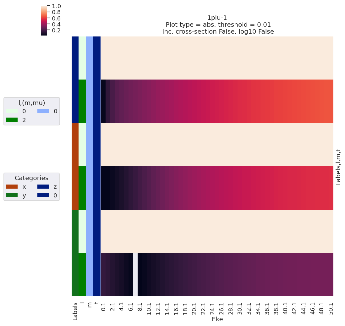
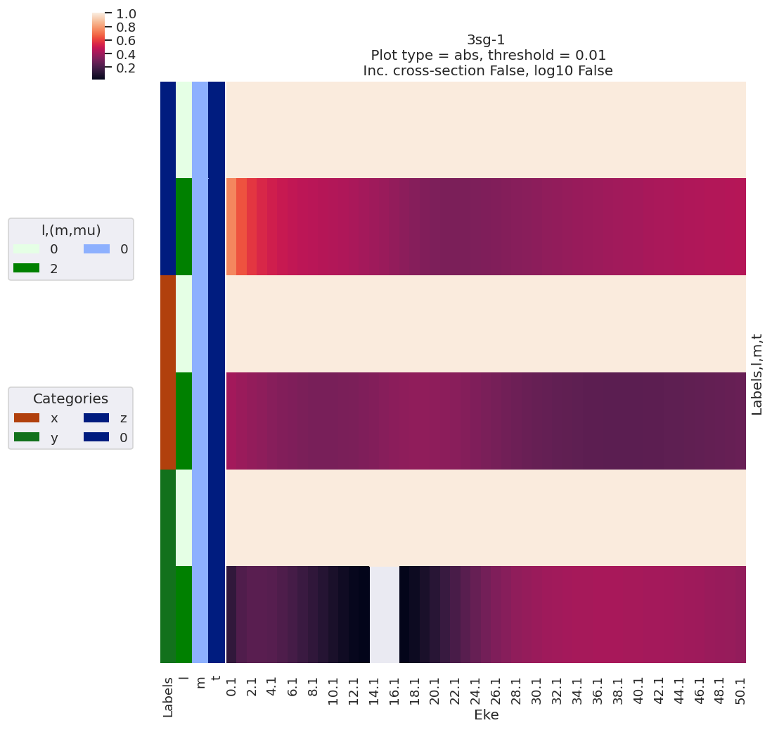
Matrix element plotting
For a full view of the computational results, use the lmPlot() method with the default, which correspond to dataType=matE.
[22]:
data.lmPlot()
Plotting data n2_1pu_0.1-50.1eV_A2.inp.out, pType=a, thres=0.01, with Seaborn
Plotting data n2_3sg_0.1-50.1eV_A2.inp.out, pType=a, thres=0.01, with Seaborn
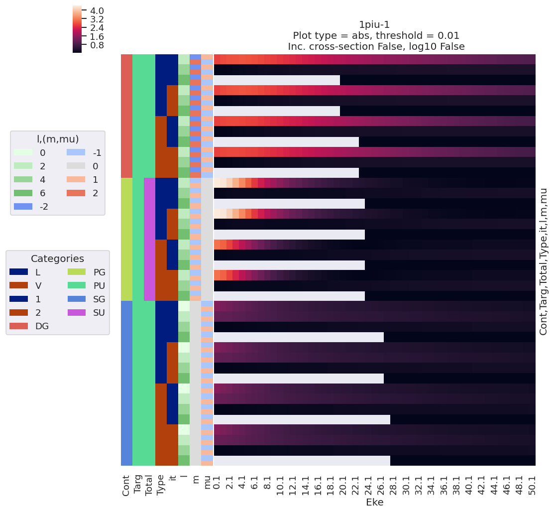
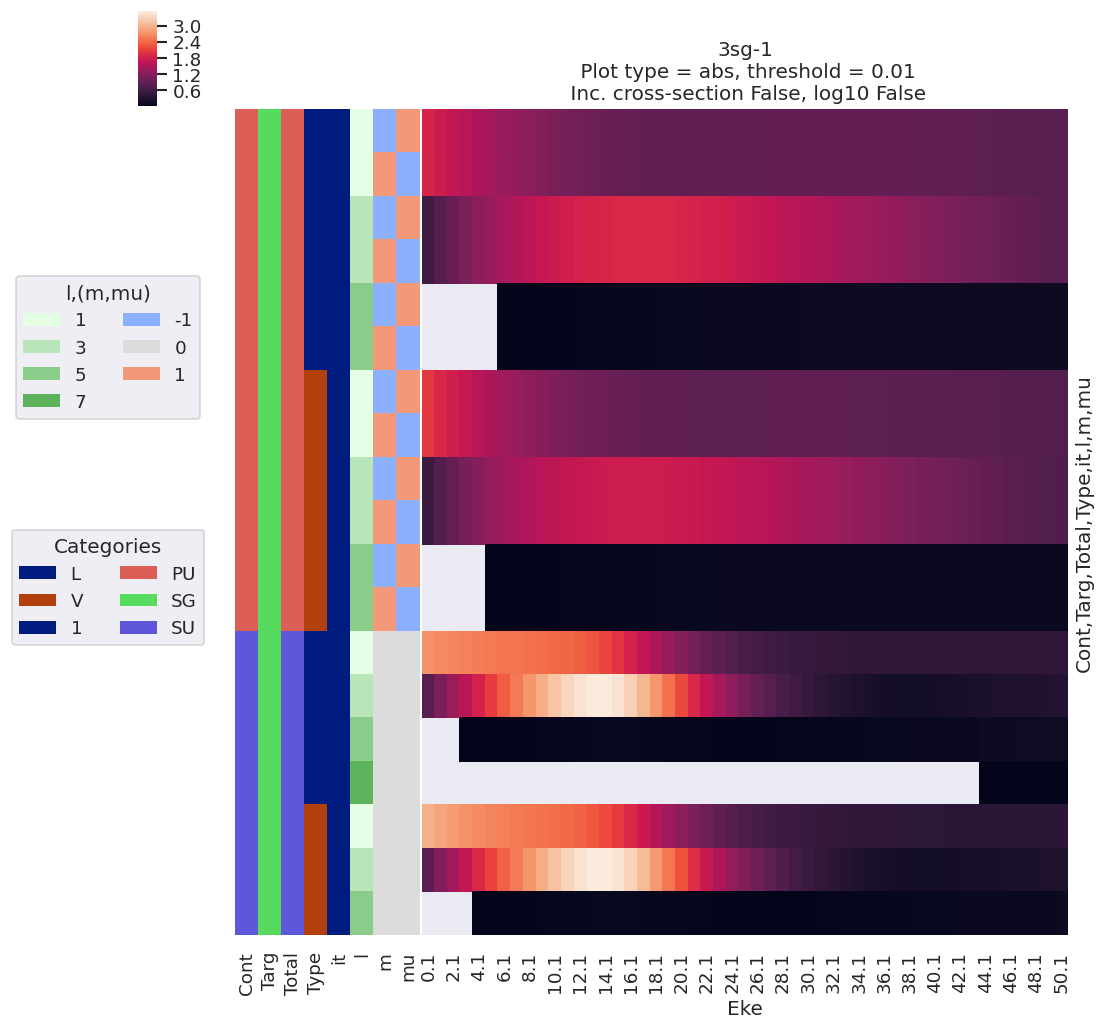
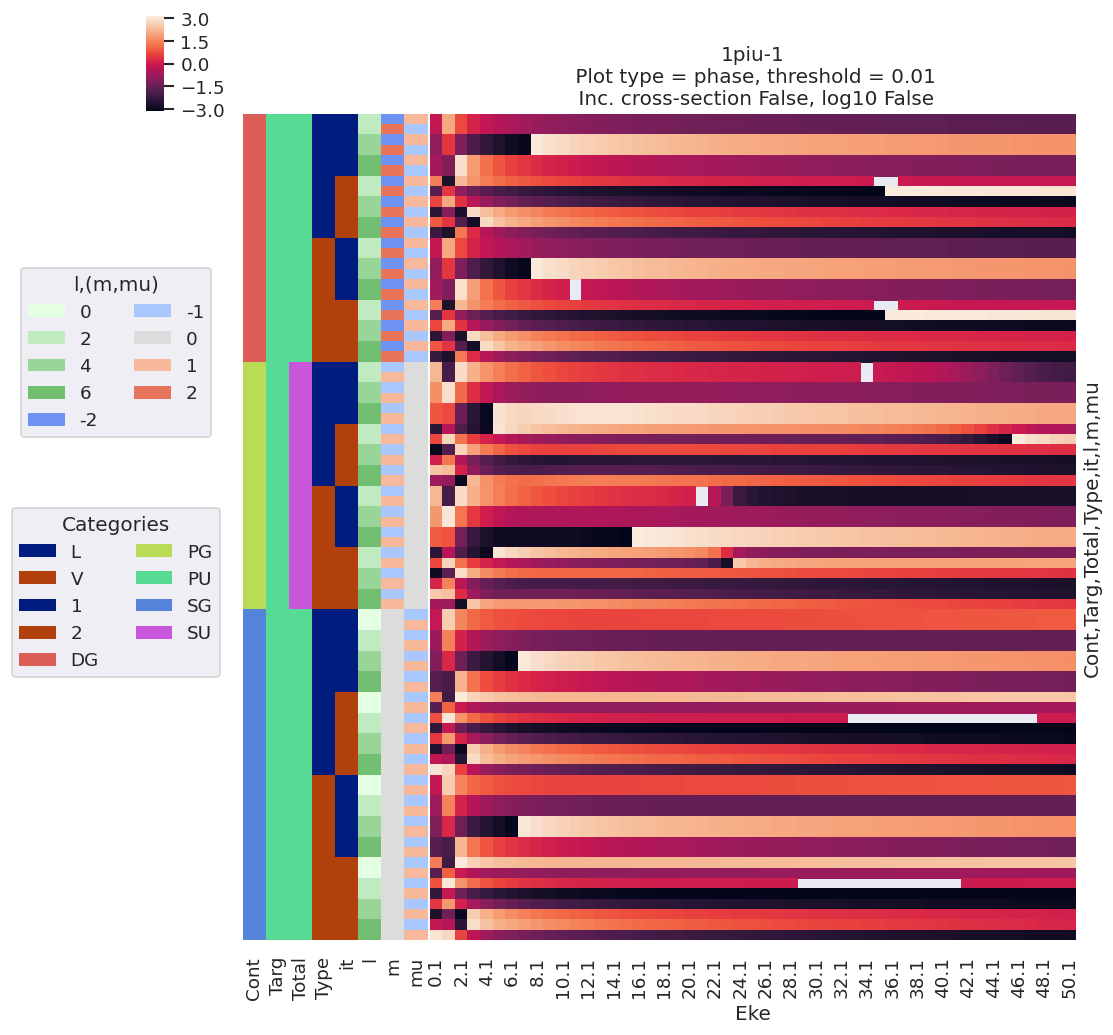
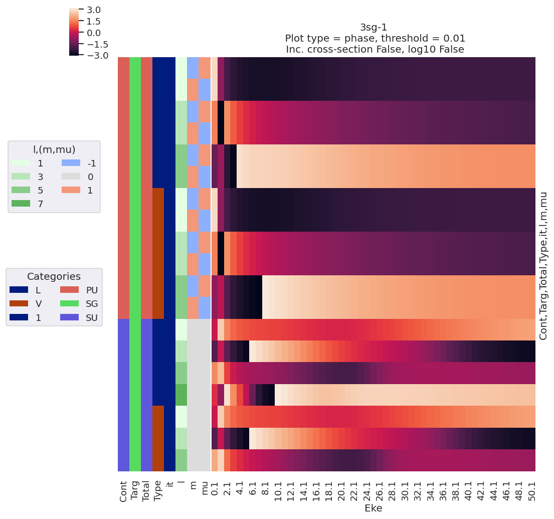
The default here plots abs values, but the same routine can be set for phase plotting.
[23]:
data.lmPlot(pType='phase')
Plotting data n2_1pu_0.1-50.1eV_A2.inp.out, pType=phase, thres=0.01, with Seaborn
Plotting data n2_3sg_0.1-50.1eV_A2.inp.out, pType=phase, thres=0.01, with Seaborn
Versions
[24]:
import scooby
scooby.Report(additional=['epsproc', 'xarray', 'jupyter'])
[24]:
| Tue Oct 20 15:57:33 2020 Eastern Daylight Time | |||||
| OS | Windows | CPU(s) | 32 | Machine | AMD64 |
| Architecture | 64bit | RAM | 63.9 GB | Environment | Jupyter |
| Python 3.7.3 (default, Apr 24 2019, 15:29:51) [MSC v.1915 64 bit (AMD64)] | |||||
| epsproc | 1.3.0-dev | xarray | 0.15.0 | jupyter | Version unknown |
| numpy | 1.19.2 | scipy | 1.3.0 | IPython | 7.12.0 |
| matplotlib | 3.3.1 | scooby | 0.5.6 | ||
| Intel(R) Math Kernel Library Version 2020.0.0 Product Build 20191125 for Intel(R) 64 architecture applications | |||||