Method development for geometric functions pt 3: \(\beta\) aligned-frame (AF) parameters with geometric functions.
- 09/06/20 v1
Aims:
- Develop \(\beta_{L,M}\) formalism for AF, using geometric tensor formalism as already applied to MF case.
- Develop corresponding numerical methods - see pt 1 notebook.
- Analyse geometric terms - see pt 1 notebook.
\(\beta_{L,M}^{AF}\) rewrite
The various terms defined in pt 1 can be used to redefine the full AF observables, expressed as a set of \(\beta_{L,M}\) coefficients (with the addition of another tensor to define the alignment terms).
The original (full) form for the AF equations, as implemented in ``ePSproc.afblm` <https://epsproc.readthedocs.io/en/dev/modules/epsproc.AFBLM.html>`__ (note, however, that the previous implementation is not fully tested, since it was s…l…o…w… the geometric version should avoid this issue):
Where \(I_{l,m,\mu}^{p_{i}\mu_{i},p_{f}\mu_{f}}(E)\) are the energy-dependent dipole matrix elements, and \(A_{Q,S}^{K}(t)\) define the alignment parameters.
In terms of the geometric parameters, this can be rewritten as:
Where there’s a new alignment tensor:
And the the \(\Lambda_{R',R}\) term is a simplified form of the previously derived MF term:
All phase conventions should be as the MF case, and the numerics for all the ternsors can be used as is… hopefully…
Refs for the full AF-PAD formalism above: 1. Reid, Katharine L., and Jonathan G. Underwood. “Extracting Molecular Axis Alignment from Photoelectron Angular Distributions.” The Journal of Chemical Physics 112, no. 8 (2000): 3643. https://doi.org/10.1063/1.480517. 2. Underwood, Jonathan G., and Katharine L. Reid. “Time-Resolved Photoelectron Angular Distributions as a Probe of Intramolecular Dynamics: Connecting the Molecular Frame and the Laboratory Frame.” The Journal of Chemical Physics 113, no. 3 (2000): 1067. https://doi.org/10.1063/1.481918. 3. Stolow, Albert, and Jonathan G. Underwood. “Time-Resolved Photoelectron Spectroscopy of Non-Adiabatic Dynamics in Polyatomic Molecules.” In Advances in Chemical Physics, edited by Stuart A. Rice, 139:497–584. Advances in Chemical Physics. Hoboken, NJ, USA: John Wiley & Sons, Inc., 2008. https://doi.org/10.1002/9780470259498.ch6.
Where [3] has the version as per the full form above (full asymmetric top alignment distribution expansion).
To consider
- Normalisation for ADMs? Will matter in cases where abs cross-sections are valid (but not for PADs generally).
Setup
[1]:
# Imports
import numpy as np
import pandas as pd
import xarray as xr

# Special functions
# from scipy.special import sph_harm
import spherical_functions as sf
import quaternion

# Performance & benchmarking libraries
# from joblib import Memory
# import xyzpy as xyz
import numba as nb

# Timings with ttictoc or time
# https://github.com/hector-sab/ttictoc
from ttictoc import TicToc
import time

# Package fns.
# For module testing, include path to module here
import sys
import os
modPath = r'D:\code\github\ePSproc'  # Win test machine
# modPath = r'/home/femtolab/github/ePSproc/'  # Linux test machine
sys.path.append(modPath)
import epsproc as ep
# TODO: tidy this up!
from epsproc.util import matEleSelector
from epsproc.geomFunc import geomCalc
* pyevtk not found, VTK export not available.
[2]:
from IPython.core.interactiveshell import InteractiveShell
InteractiveShell.ast_node_interactivity = "all"
Alignment terms
Axis distribution moments
These are already set up by setADMs().
[3]:
# set default alignment terms - single term A(0,0,0)=1, which corresponds to isotropic distributions
AKQS = ep.setADMs()

AKQS
[3]:
<xarray.DataArray (ADM: 1, t: 1)>
array([[1]])
Coordinates:
  * ADM      (ADM) MultiIndex
  - K        (ADM) int64 0
  - Q        (ADM) int64 0
  - S        (ADM) int64 0
  * t        (t) int32 0
Attributes:
    dataType:  ADM
[4]:
AKQSpd,_ = ep.util.multiDimXrToPD(AKQS, colDims='t', squeeze=False)
AKQSpd
[4]:
| t | 0 | ||
|---|---|---|---|
| K | Q | S | |
| 0 | 0 | 0 | 1 |
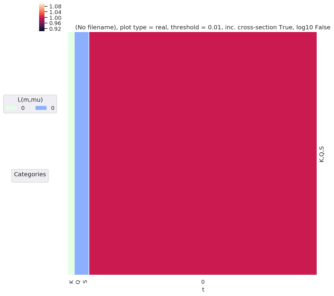
[5]:
daPlot, daPlotpd, legendList, gFig = ep.lmPlot(AKQS, xDim = 't', pType = 'r', squeeze = False)  # Note squeeze = False required for 1D case (should add this to code!)
daPlotpd
Plotting data (No filename), pType=r, thres=0.01, with Seaborn
No handles with labels found to put in legend.
[5]:
| t | 0 | ||
|---|---|---|---|
| K | Q | S | |
| 0 | 0 | 0 | 1.0 |
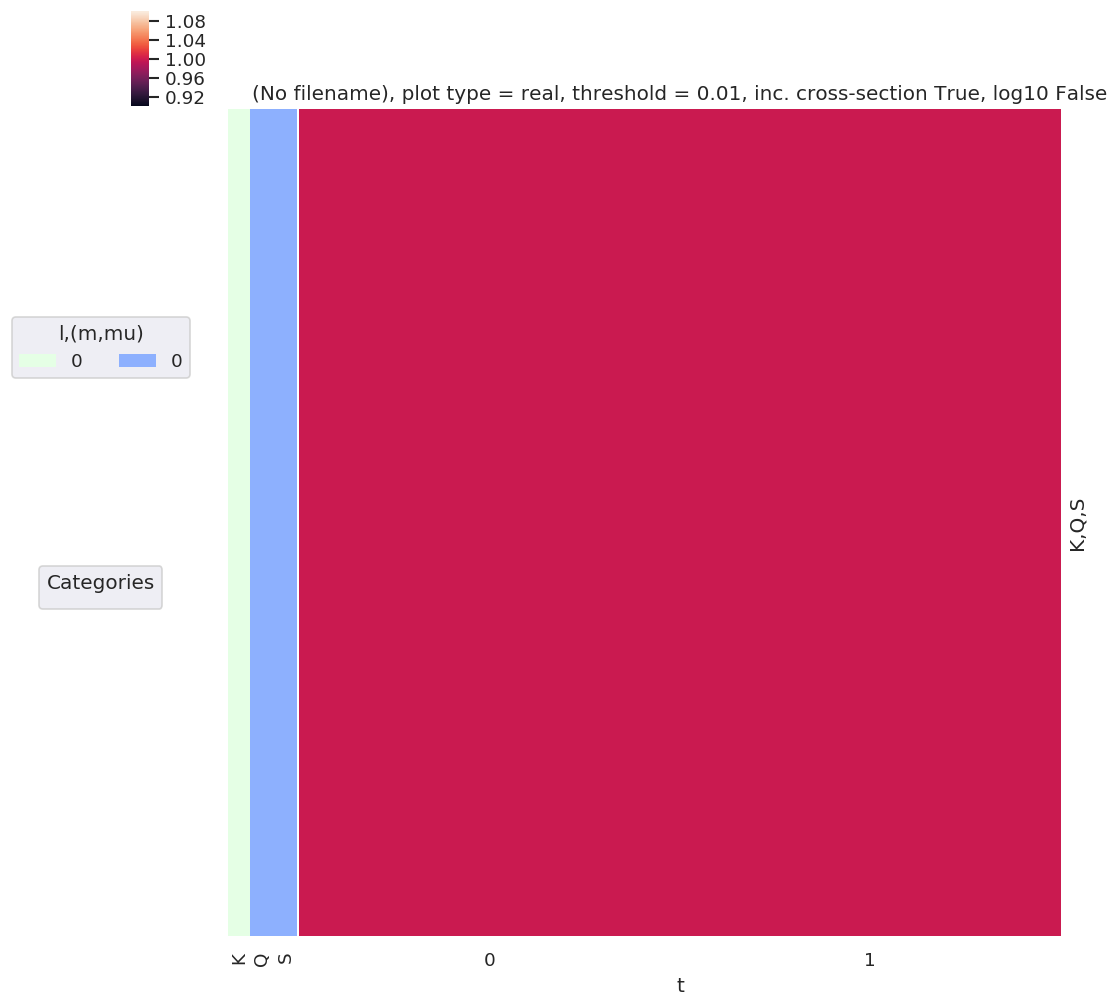
[6]:
# Test multiple t points
AKQS = ep.setADMs(ADMs = [0,0,0,1,1], t=[0,1])
daPlot, daPlotpd, legendList, gFig = ep.lmPlot(AKQS, xDim = 't', pType = 'r', squeeze = False)  # Note squeeze = False required for 1D case (should add this to code!)
daPlotpd
Plotting data (No filename), pType=r, thres=0.01, with Seaborn
No handles with labels found to put in legend.
[6]:
| t | 0 | 1 | ||
|---|---|---|---|---|
| K | Q | S | ||
| 0 | 0 | 0 | 1.0 | 1.0 |
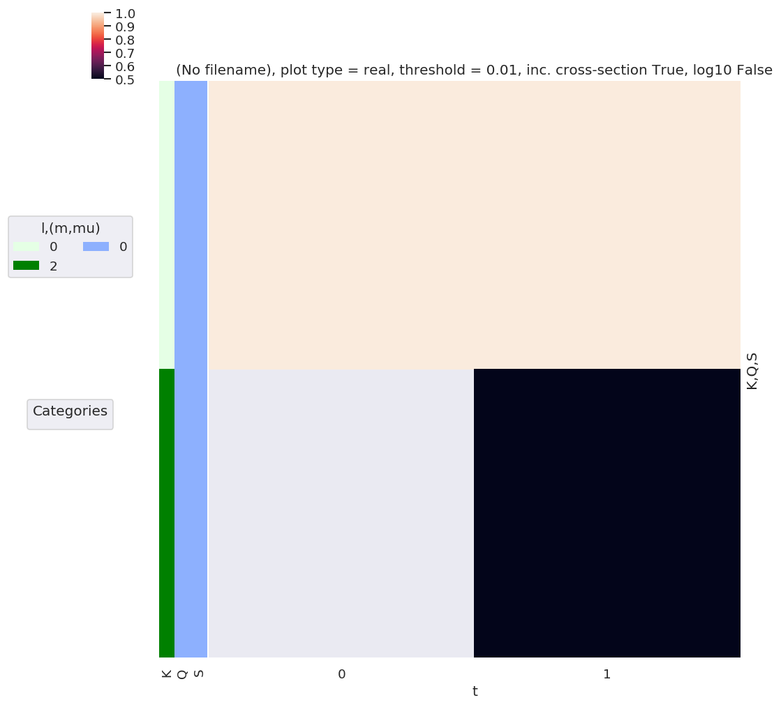
[7]:
# Test additional time-dependent values
AKQS = ep.setADMs(ADMs = [[0,0,0,1,1],[2,0,0,0,0.5]], t=[0,1])    # Nested list or np.array OK.
# AKQS = ep.setADMs(ADMs = np.array([[0,0,0,1,1],[2,0,0,0,0.5]]), t=[0,1])
daPlot, daPlotpd, legendList, gFig = ep.lmPlot(AKQS, xDim = 't', pType = 'r', squeeze = False)  # Note squeeze = False required for 1D case (should add this to code!)
daPlotpd
No handles with labels found to put in legend.
Plotting data (No filename), pType=r, thres=0.01, with Seaborn
[7]:
| t | 0 | 1 | ||
|---|---|---|---|---|
| K | Q | S | ||
| 0 | 0 | 0 | 1.0 | 1.0 |
| 2 | 0 | 0 | NaN | 0.5 |
Alignment tensor
As previously defined:
Function dev
Based on existing MF functions, see ep.geomFunc.geomCalc and ep.geomFunc.mfblmGeom.
Most similar to existing betaTerm() function, which also has product of 3j terms in a similar manner.
[8]:
# Generate QNs - code adapted from ep.geomFunc.geomUtils.genllL(Lmin = 0, Lmax = 10, mFlag = True):

# Generate QNs for deltaKQS term - 3j product term
def genKQSterms(Kmin = 0, Kmax = 2, mFlag = True):
    # Set QNs for calculation, (l,m,mp)
    QNs = []
    for P in np.arange(0, 2+1):    # HARD-CODED R for testing - should get from EPR tensor defn. in full calcs.
        for K in np.arange(Kmin, Kmax+1):  # Eventually this will come from alignment term
            for L in np.arange(np.abs(P-K), P+K+1):  # Allowed L given P and K defined

                if mFlag:    # Include "m" (or equivalent) terms?
                    mMax = L
                    RMax = P
                    QMax = K
                else:
                    mMax = 0
                    RMax = 0
                    QMax = 0

                for R in np.arange(-RMax, RMax+1):
                    for Q in np.arange(-QMax, QMax+1):
                        #for M in np.arange(np.abs(l-lp), l+lp+1):
#                         for M in np.arange(-mMax, mMax+1):
                            # Set M - note this implies specific phase choice.
                            # M = -(m+mp)
                            # M = (-m+mp)
                            # if np.abs(M) <= L:  # Skip terms with invalid M
                            #     QNs.append([l, lp, L, m, mp, M])

                        # Run for all possible M
                        for M in np.arange(-L, L+1):
                            QNs.append([P, K, L, R, Q, M])

    return np.array(QNs)


# Generate QNs from EPR + AKQS tensors
def genKQStermsFromTensors(EPR, AKQS, uniqueFlag = True, phaseConvention = 'S'):
    '''
    Generate all QNs for :math:`\Delta_{L,M}(K,Q,S)` from existing tensors (Xarrays) :math:`E_{P,R}` and :math:`A^K_{Q,S}`.

    Cf. :py:func:`epsproc.geomFunc.genllpMatE`, code adapted from there.

    Parameters
    ----------
    matE : Xarray
        Xarray containing matrix elements, with QNs (l,m), as created by :py:func:`readMatEle`

    uniqueFlag : bool, default = True
        Check for duplicates and remove (can occur with some forms of matrix elements).

    mFlag : bool, optional, default = True
        m, mp take all passed values if mFlag=True, or =0 only if mFlag=False

    phaseConvention : optional, str, default = 'S'
        Set phase conventions with :py:func:`epsproc.geomCalc.setPhaseConventions`.
        To use preset phase conventions, pass existing dictionary.
        If matE.attrs['phaseCons'] is already set, this will be used instead of passed args.


    Returns
    -------
    QNs1, QNs2 : two 2D np.arrays
        Values take all allowed combinations ['P','K','L','R','Q','M'] and ['P','K','L','Rp','S','S-Rp'] from supplied matE.
        Note phase conventions not applied to QN lists as yet.

    To do
    -----
    - Implement output options (see dev. function w3jTable).

    '''

    # Local import.
    from epsproc.geomFunc.geomCalc import setPhaseConventions

    # For transparency/consistency with subfunctions, str/dict now set in setPhaseConventions()
    if 'phaseCons' in EPR.attrs.keys():
        phaseCons = EPR.attrs['phaseCons']
    else:
        phaseCons = setPhaseConventions(phaseConvention = phaseConvention)

    # Get QNs from inputs
    KQScoords = AKQS.unstack().coords  # Use unstack here, or np.unique(matE.l), to avoid duplicates
    PRcoords = EPR.unstack().coords

    # Use passed (m,mp) values, or run for m=mp=0 only.
#     if mFlag:
#         mList = matE.unstack().m.values
#     else:
#         mList = 0

    # Set QNs for calculation, one set for each 3j term
    QNs1 = []
    QNs2 = []
    for P in PRcoords['P'].values:   # Note dictionary syntax for coords objects
        for K in KQScoords['K'].values:
            for L in np.arange(np.abs(P-K), P+K+1):  # Allowed L given P and K defined

#                 if mFlag:    # Include "m" (or equivalent) terms?
#                     mMax = L
#                     RMax = P
#                     QMax = K
#                 else:
#                     mMax = 0
#                     RMax = 0
#                     QMax = 0

                for R in PRcoords['R'].values:
                    for Q in KQScoords['Q'].values:

                        # Set M, with +/- phase convention - TBC MAY BE INCORRECT IN THIS CASE/CONTEXT?
                        # Note that setting phaseCons['afblmCons']['negM']  = phaseCons['genMatEcons']['negm'] is current default case, but doesn't have to be!
                        if phaseCons['genMatEcons']['negm']:
                            M = (-R+Q)  # Case for M -> -M switch
                        else:
                            M = -(R+Q)  # Usual phase convention.

                        QNs1.append([P, K, L, R, Q, M])

                # Set Rp and S - these are essentially independent of R,Q,M, but keep nested for full dim output.
                for Rp in PRcoords['R'].values:
                    for S in KQScoords['S'].values:
                        SRp = S-Rp  # Set final 3j term, S-Rp

                        QNs2.append([P, K, L, Rp, S, SRp])

                            #for M in np.arange(np.abs(l-lp), l+lp+1):
    #                         for M in np.arange(-mMax, mMax+1):
                                # Set M - note this implies specific phase choice.
                                # M = -(m+mp)
                                # M = (-m+mp)
                                # if np.abs(M) <= L:  # Skip terms with invalid M
                                #     QNs.append([l, lp, L, m, mp, M])

                            # Run for all possible M
    #                         for M in np.arange(-L, L+1):
    #                             QNs.append([P, K, L, R, Q, M])


    if uniqueFlag:
        return np.unique(QNs1, axis = 0), np.unique(QNs2, axis = 0)
    else:
        return np.array(QNs1), np.array(QNs2)
[9]:
test = genKQSterms()
# test.tolist()   # Use tolist() to get full array output (not truncated by np)
test.shape
[9]:
(1225, 6)
[10]:
# Can also just use existing fn.
test2 = ep.geomFunc.genllL(Lmax=2)
test2.shape
[10]:
(1225, 6)
[11]:
# Also QN list fn - checks and removes duplicates
QNs = ep.geomFunc.genllL(Lmax=2)
test3 = ep.geomFunc.geomUtils.genllLList(QNs, uniqueFlag = True, mFlag = True)

test3.shape
[11]:
(1225, 6)
All QNs
[12]:
# Then calc 3js.... as per betaTerm
form = 'xdaLM'  # xds
dlist1 = ['P', 'K', 'L', 'R', 'Q', 'M']
dlist2 = ['P', 'K', 'L', 'Rp', 'S', 'S-Rp']

QNs = ep.geomFunc.genllL(Lmax=2)
[13]:
# Set phase conventions for this case, extending existing structure
phaseCons = ep.geomFunc.setPhaseConventions('E')

phaseCons['afblmCons'] = {}

# (+/-)M phase selection, set as per existing code, betaCons['negM'] = genMatEcons['negm']       # Use -M term in 3j? Should be anti-correlated with genMatEcons['negm']...? 31/03/20 NOW correlated with mfblmCons['Mphase']
# Note this is correlated with QN generation in genllpMatE() - should set equivalent fn for alignment terms.
# In existing case this arises from M = (-m+mp) or M = -(m+mp) choice.
phaseCons['afblmCons']['negM'] = phaseCons['genMatEcons']['negm']
phaseCons['afblmCons']['negQ'] = True
phaseCons['afblmCons']['negS'] = True


# Apply phase conventions to input QNs
#         if phaseCons['mfblmCons']['BLMmPhase']:
#             QNsBLMtable[:,3] *= -1
#             QNsBLMtable[:,5] *= -1
[14]:
# Calculate two 3j terms, with respective QN sets
thrj1 = ep.geomFunc.w3jTable(QNs = QNs, nonzeroFlag = True, form = form, dlist = dlist1)
thrj2 = ep.geomFunc.w3jTable(QNs = QNs, nonzeroFlag = True, form = form, dlist = dlist2)
[15]:
# Multiplication term...

testMult = thrj1.unstack() * thrj2.unstack()

# This can get large quickly - for Kmax=2 already have 2e6 terms
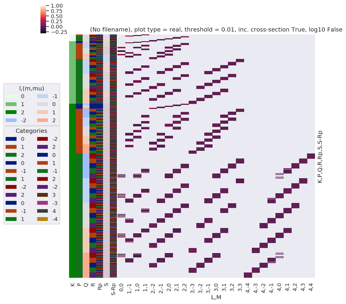
[16]:
# plotDimsRed = ['l', 'm', 'lp', 'mp']
xDim = {'LM':['L','M']}
# daPlot, daPlotpd, legendList, gFig = ep.lmPlot(testMult, plotDims=plotDimsRed, xDim=xDim, pType = 'r')
daPlot, daPlotpd, legendList, gFig = ep.lmPlot(testMult, xDim=xDim, pType = 'r')
Set dataType (No dataType)
Plotting data (No filename), pType=r, thres=0.01, with Seaborn
C:\Users\femtolab\.conda\envs\ePSdev\lib\site-packages\xarray\core\nputils.py:215: RuntimeWarning:

All-NaN slice encountered
Reduced QNs set
[17]:
# Then calc 3js.... as per betaTerm
form = 'xdaLM'  # xds
dlist1 = ['P', 'K', 'L', 'R', 'Q', 'M']
dlist2 = ['P', 'K', 'L', 'Rp', 'S', 'S-Rp']

# Calculate two 3j terms, with respective QN sets
thrj1 = ep.geomFunc.w3jTable(QNs = QNs, nonzeroFlag = True, form = form, dlist = dlist1)
thrj2 = ep.geomFunc.w3jTable(QNs = QNs, nonzeroFlag = True, form = form, dlist = dlist2)
[18]:
# With subselection (currently don't have QN generation fnc of correct form - see geomUtils)
# from epsproc.util import matEleSelector
# thrj1Sel = ep.util.matEleSelector(thrj1, inds = {'Q':0}, sq=False)
[19]:
# Check 3j terms
xDim = {'LM':['L','M']}
daPlot, daPlotpd, legendList, gFig = ep.lmPlot(thrj1, xDim=xDim, pType = 'r')
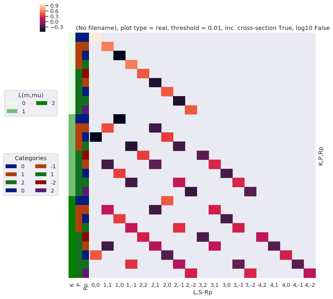
xDim = {'LM':['L','S-Rp']}
daPlot, daPlotpd, legendList, gFig = ep.lmPlot(thrj2.sel({'S':0}), xDim=xDim, pType = 'r')
C:\Users\femtolab\.conda\envs\ePSdev\lib\site-packages\xarray\core\nputils.py:215: RuntimeWarning:

All-NaN slice encountered
Plotting data (No filename), pType=r, thres=0.01, with Seaborn
C:\Users\femtolab\.conda\envs\ePSdev\lib\site-packages\xarray\core\nputils.py:215: RuntimeWarning:

All-NaN slice encountered
Plotting data (No filename), pType=r, thres=0.01, with Seaborn
[20]:
# Multiplication term...

testMultSub = thrj1.unstack().sel({'Q':0}) * thrj2.unstack().sel({'S':0})   # SLOW, 91125 elements. ACTUALLY - much faster after a reboot. Sigh.

testMultSub2 = thrj1.sel({'Q':0}).unstack() * thrj2.sel({'S':0}).unstack()  # FAST, 28125 elements. Possible issue with which dims are dropped - check previous notes!

# This can get large quickly - for Kmax=2 already have 2e6 terms

testMultSub.notnull().sum() # == 194 for Kmax = 2, Q=S=0
testMultSub2.notnull().sum() # == 194 for Kmax = 2, Q=S=0  OK
[20]:
<xarray.DataArray 'w3jStacked' ()>
array(194)
Coordinates:
    Q        int64 0
    S        int64 0
[20]:
<xarray.DataArray 'w3jStacked' ()>
array(194)
[21]:
# plotDimsRed = ['l', 'm', 'lp', 'mp']
xDim = {'LM':['L','M']}
# daPlot, daPlotpd, legendList, gFig = ep.lmPlot(testMult, plotDims=plotDimsRed, xDim=xDim, pType = 'r')
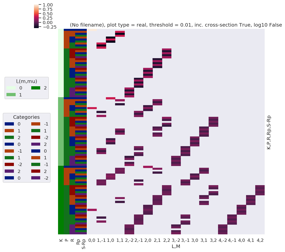
daPlot, daPlotpd, legendList, gFig = ep.lmPlot(testMultSub, xDim=xDim, pType = 'r')
Set dataType (No dataType)
Plotting data (No filename), pType=r, thres=0.01, with Seaborn
C:\Users\femtolab\.conda\envs\ePSdev\lib\site-packages\xarray\core\nputils.py:215: RuntimeWarning:

All-NaN slice encountered
[22]:
# plotDimsRed = ['l', 'm', 'lp', 'mp']
xDim = {'LM':['L','M']}
# daPlot, daPlotpd, legendList, gFig = ep.lmPlot(testMult, plotDims=plotDimsRed, xDim=xDim, pType = 'r')
daPlot, daPlotpd, legendList, gFig = ep.lmPlot(testMultSub2, xDim=xDim, pType = 'r')
Set dataType (No dataType)
Plotting data (No filename), pType=r, thres=0.01, with Seaborn
C:\Users\femtolab\.conda\envs\ePSdev\lib\site-packages\xarray\core\nputils.py:215: RuntimeWarning:

All-NaN slice encountered
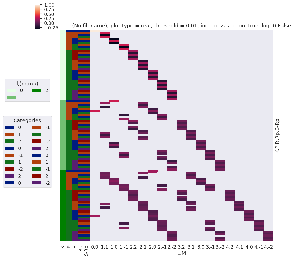
Plots appear to be the same, aside from ordering of M terms(?)
QNs from existing tensors
[23]:
phaseConvention = 'E'

# Set polarisation term
p=[0]
EPRX = geomCalc.EPR(form = 'xarray', p = p, nonzeroFlag = True, phaseConvention = phaseConvention).unstack().sel({'R-p':0}).drop('R-p') # Set for R-p = 0 for p=0 case (redundant coord) - need to fix in e-field mult term!
EPRXresort = EPRX.squeeze(['l','lp']).drop(['l','lp'])  # Safe squeeze & drop of selected singleton dims only.

# Set alignment terms (inc. time-dependence)
AKQS = ep.setADMs(ADMs = [[0,0,0,1,1],[2,0,0,0,0.5]], t=[0,1])    # Nested list or np.array OK.
[24]:
# Calculate alignment term - this cell should form core function, cf. betaTerm() etc.

# Set QNs
QNs1, QNs2 = genKQStermsFromTensors(EPRXresort, AKQS, uniqueFlag = True, phaseConvention = phaseConvention)

# Then calc 3js.... as per betaTerm
form = 'xdaLM'  # xds
dlist1 = ['P', 'K', 'L', 'R', 'Q', 'M']
dlist2 = ['P', 'K', 'L', 'Rp', 'S', 'S-Rp']

# Copy QNs and apply any additional phase conventions
QNs1DeltaTable = QNs1.copy()
QNs2DeltaTable = QNs2.copy()

# Set additional phase cons here - these will be set in master function eventually!
# NOTE - only testing for Q=S=0 case initially.
phaseCons['afblmCons']['negM'] = phaseCons['genMatEcons']['negm']  # IF SET TO TRUE THIS KNOCKS OUT M!=0 terms - not sure if this is correct here, depends also on phase cons in genKQStermsFromTensors().
                                                                    # Yeah, looks like phase error in current case, get terms with R=M, instead of R=-M
                                                                    # Confusion is due to explicit assignment of +/-M terms in QN generation (only allowed terms), which *already* enforces this phase convention.
phaseCons['afblmCons']['negQ'] = True
phaseCons['afblmCons']['negS'] = True

# Switch signs (m,M) before 3j calcs.
if phaseCons['afblmCons']['negQ']:
    QNs1DeltaTable[:,4] *= -1

# Switch sign Q > -Q before 3j calcs.
if phaseCons['afblmCons']['negM']:
    QNs1DeltaTable[:,5] *= -1

# Switch sign S > -S before 3j calcs.
if phaseCons['afblmCons']['negS']:
    QNs2DeltaTable[:,4] *= -1


# Calculate two 3j terms, with respective QN sets
thrj1 = ep.geomFunc.w3jTable(QNs = QNs1DeltaTable, nonzeroFlag = True, form = form, dlist = dlist1)
thrj2 = ep.geomFunc.w3jTable(QNs = QNs2DeltaTable, nonzeroFlag = True, form = form, dlist = dlist2)

# Multiply
thrjMult = thrj1.unstack() * thrj2.unstack()

# Additional terms & multiplications
Kdegen = np.sqrt(2*thrjMult.K + 1)
KQphase = np.power(-1, np.abs(thrjMult.K + thrjMult.Q))

DeltaKQS =  Kdegen * KQphase * thrjMult

# AF term
AFterm = (DeltaKQS * AKQS.unstack()).sum({'K','Q','S'})
[25]:
thrjMult.notnull().sum() # == 69 for test case with all phase switches on, and same for no phase switches (in test case Q=S=0 in any case!)
[25]:
<xarray.DataArray 'w3jStacked' ()>
array(69)
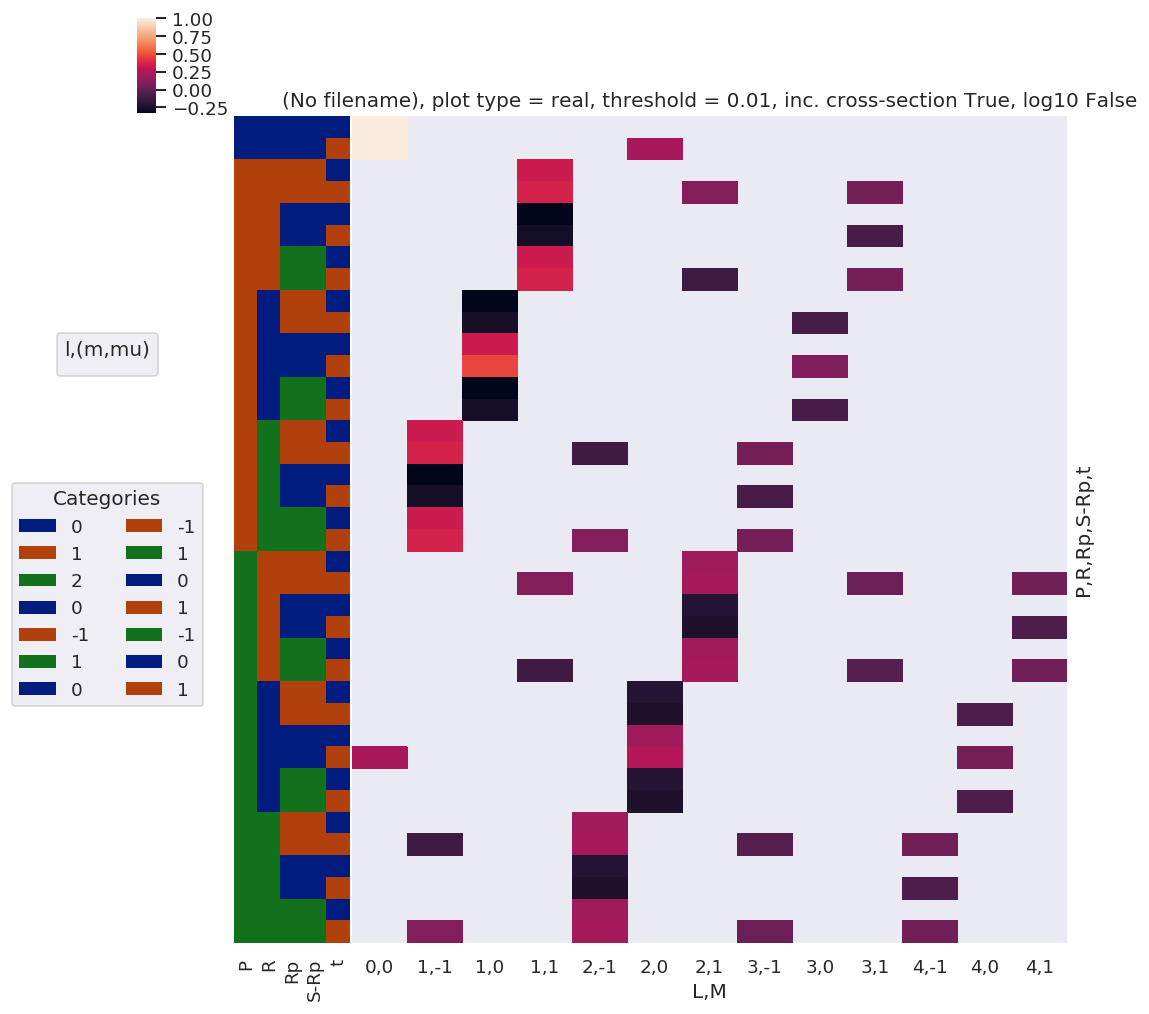
[26]:
# Plot
xDim = {'LM':['L','M']}
# daPlot, daPlotpd, legendList, gFig = ep.lmPlot(testMult, plotDims=plotDimsRed, xDim=xDim, pType = 'r')
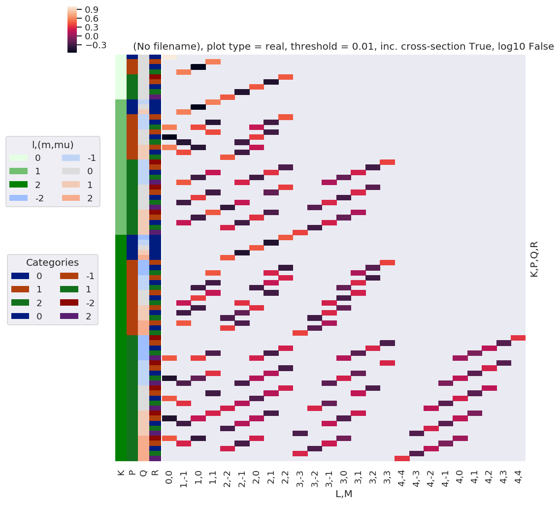
daPlot, daPlotpd, legendList, gFig = ep.lmPlot(DeltaKQS, xDim=xDim, pType = 'r')
Set dataType (No dataType)
Plotting data (No filename), pType=r, thres=0.01, with Seaborn
C:\Users\femtolab\.conda\envs\ePSdev\lib\site-packages\xarray\core\nputils.py:215: RuntimeWarning:

All-NaN slice encountered
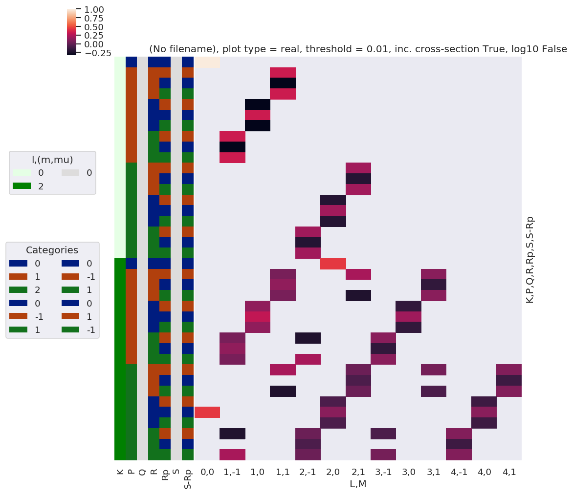
[27]:
# Plot
xDim = {'LM':['L','M']}
# daPlot, daPlotpd, legendList, gFig = ep.lmPlot(testMult, plotDims=plotDimsRed, xDim=xDim, pType = 'r')
daPlot, daPlotpd, legendList, gFig = ep.lmPlot(AFterm, xDim=xDim, pType = 'r')
daPlotpd
Set dataType (No dataType)
Plotting data (No filename), pType=r, thres=0.01, with Seaborn
No handles with labels found to put in legend.
[27]:
| L | 0 | 1 | 2 | 3 | 4 | ||||||||||||
|---|---|---|---|---|---|---|---|---|---|---|---|---|---|---|---|---|---|
| M | 0 | -1 | 0 | 1 | -1 | 0 | 1 | -1 | 0 | 1 | -1 | 0 | 1 | ||||
| P | R | Rp | S-Rp | t | |||||||||||||
| 0 | 0 | 0 | 0 | 0 | 1.000000 | NaN | NaN | NaN | NaN | NaN | NaN | NaN | NaN | NaN | NaN | NaN | NaN |
| 1 | 1.000000 | NaN | NaN | NaN | NaN | 0.223607 | NaN | NaN | NaN | NaN | NaN | NaN | NaN | ||||
| 1 | -1 | -1 | 1 | 0 | NaN | NaN | NaN | 0.333333 | NaN | NaN | NaN | NaN | NaN | NaN | NaN | NaN | NaN |
| 1 | NaN | NaN | NaN | 0.370601 | NaN | NaN | 0.111803 | NaN | NaN | 0.063888 | NaN | NaN | NaN | ||||
| 0 | 0 | 0 | NaN | NaN | NaN | -0.333333 | NaN | NaN | NaN | NaN | NaN | NaN | NaN | NaN | NaN | ||
| 1 | NaN | NaN | NaN | -0.258798 | NaN | NaN | NaN | NaN | NaN | -0.078246 | NaN | NaN | NaN | ||||
| 1 | -1 | 0 | NaN | NaN | NaN | 0.333333 | NaN | NaN | NaN | NaN | NaN | NaN | NaN | NaN | NaN | ||
| 1 | NaN | NaN | NaN | 0.370601 | NaN | NaN | -0.111803 | NaN | NaN | 0.063888 | NaN | NaN | NaN | ||||
| 0 | -1 | 1 | 0 | NaN | NaN | -0.333333 | NaN | NaN | NaN | NaN | NaN | NaN | NaN | NaN | NaN | NaN | |
| 1 | NaN | NaN | -0.258798 | NaN | NaN | NaN | NaN | NaN | -0.078246 | NaN | NaN | NaN | NaN | ||||
| 0 | 0 | 0 | NaN | NaN | 0.333333 | NaN | NaN | NaN | NaN | NaN | NaN | NaN | NaN | NaN | NaN | ||
| 1 | NaN | NaN | 0.482405 | NaN | NaN | NaN | NaN | NaN | 0.095831 | NaN | NaN | NaN | NaN | ||||
| 1 | -1 | 0 | NaN | NaN | -0.333333 | NaN | NaN | NaN | NaN | NaN | NaN | NaN | NaN | NaN | NaN | ||
| 1 | NaN | NaN | -0.258798 | NaN | NaN | NaN | NaN | NaN | -0.078246 | NaN | NaN | NaN | NaN | ||||
| 1 | -1 | 1 | 0 | NaN | 0.333333 | NaN | NaN | NaN | NaN | NaN | NaN | NaN | NaN | NaN | NaN | NaN | |
| 1 | NaN | 0.370601 | NaN | NaN | -0.111803 | NaN | NaN | 0.063888 | NaN | NaN | NaN | NaN | NaN | ||||
| 0 | 0 | 0 | NaN | -0.333333 | NaN | NaN | NaN | NaN | NaN | NaN | NaN | NaN | NaN | NaN | NaN | ||
| 1 | NaN | -0.258798 | NaN | NaN | NaN | NaN | NaN | -0.078246 | NaN | NaN | NaN | NaN | NaN | ||||
| 1 | -1 | 0 | NaN | 0.333333 | NaN | NaN | NaN | NaN | NaN | NaN | NaN | NaN | NaN | NaN | NaN | ||
| 1 | NaN | 0.370601 | NaN | NaN | 0.111803 | NaN | NaN | 0.063888 | NaN | NaN | NaN | NaN | NaN | ||||
| 2 | -1 | -1 | 1 | 0 | NaN | NaN | NaN | NaN | NaN | NaN | 0.200000 | NaN | NaN | NaN | NaN | NaN | NaN |
| 1 | NaN | NaN | NaN | 0.111803 | NaN | NaN | 0.215972 | NaN | NaN | 0.031944 | NaN | NaN | 0.053240 | ||||
| 0 | 0 | 0 | NaN | NaN | NaN | NaN | NaN | NaN | -0.200000 | NaN | NaN | NaN | NaN | NaN | NaN | ||
| 1 | NaN | NaN | NaN | NaN | NaN | NaN | -0.231944 | NaN | NaN | NaN | NaN | NaN | -0.058321 | ||||
| 1 | -1 | 0 | NaN | NaN | NaN | NaN | NaN | NaN | 0.200000 | NaN | NaN | NaN | NaN | NaN | NaN | ||
| 1 | NaN | NaN | NaN | -0.111803 | NaN | NaN | 0.215972 | NaN | NaN | -0.031944 | NaN | NaN | 0.053240 | ||||
| 0 | -1 | 1 | 0 | NaN | NaN | NaN | NaN | NaN | -0.200000 | NaN | NaN | NaN | NaN | NaN | NaN | NaN | |
| 1 | NaN | NaN | NaN | NaN | NaN | -0.231944 | NaN | NaN | NaN | NaN | NaN | -0.058321 | NaN | ||||
| 0 | 0 | 0 | NaN | NaN | NaN | NaN | NaN | 0.200000 | NaN | NaN | NaN | NaN | NaN | NaN | NaN | ||
| 1 | 0.223607 | NaN | NaN | NaN | NaN | 0.263888 | NaN | NaN | NaN | NaN | NaN | 0.063888 | NaN | ||||
| 1 | -1 | 0 | NaN | NaN | NaN | NaN | NaN | -0.200000 | NaN | NaN | NaN | NaN | NaN | NaN | NaN | ||
| 1 | NaN | NaN | NaN | NaN | NaN | -0.231944 | NaN | NaN | NaN | NaN | NaN | -0.058321 | NaN | ||||
| 1 | -1 | 1 | 0 | NaN | NaN | NaN | NaN | 0.200000 | NaN | NaN | NaN | NaN | NaN | NaN | NaN | NaN | |
| 1 | NaN | -0.111803 | NaN | NaN | 0.215972 | NaN | NaN | -0.031944 | NaN | NaN | 0.053240 | NaN | NaN | ||||
| 0 | 0 | 0 | NaN | NaN | NaN | NaN | -0.200000 | NaN | NaN | NaN | NaN | NaN | NaN | NaN | NaN | ||
| 1 | NaN | NaN | NaN | NaN | -0.231944 | NaN | NaN | NaN | NaN | NaN | -0.058321 | NaN | NaN | ||||
| 1 | -1 | 0 | NaN | NaN | NaN | NaN | 0.200000 | NaN | NaN | NaN | NaN | NaN | NaN | NaN | NaN | ||
| 1 | NaN | 0.111803 | NaN | NaN | 0.215972 | NaN | NaN | 0.031944 | NaN | NaN | 0.053240 | NaN | NaN | ||||
Note here that there are blocks of non-zero terms with M=+/-1, these should drop out later (?) by sums over symmetry and/or other 3j terms… TBC…
Lambda term redux
Use existing function and force/sub-select terms…
[28]:
# Code adapted from mfblmXprod()

eulerAngs = np.array([0,0,0], ndmin=2)
# RX = ep.setPolGeoms(eulerAngs = eulerAngs)   # This throws error in geomCalc.MFproj???? Something to do with form of terms passed to wD, line 970 vs. 976 in geomCalc.py
RX = ep.setPolGeoms()   # (0,0,0) term in geomCalc.MFproj OK.

lambdaTerm, lambdaTable, lambdaD, QNsLambda = geomCalc.MFproj(RX = RX, form = 'xarray', phaseConvention = phaseConvention)
# lambdaTermResort = lambdaTerm.squeeze().drop('l').drop('lp')   # This removes photon (l,lp) dims fully.
lambdaTermResort = lambdaTerm.squeeze(['l','lp']).drop(['l','lp']).sel({'Labels':'z'})  # Safe squeeze & drop of selected singleton dims only.
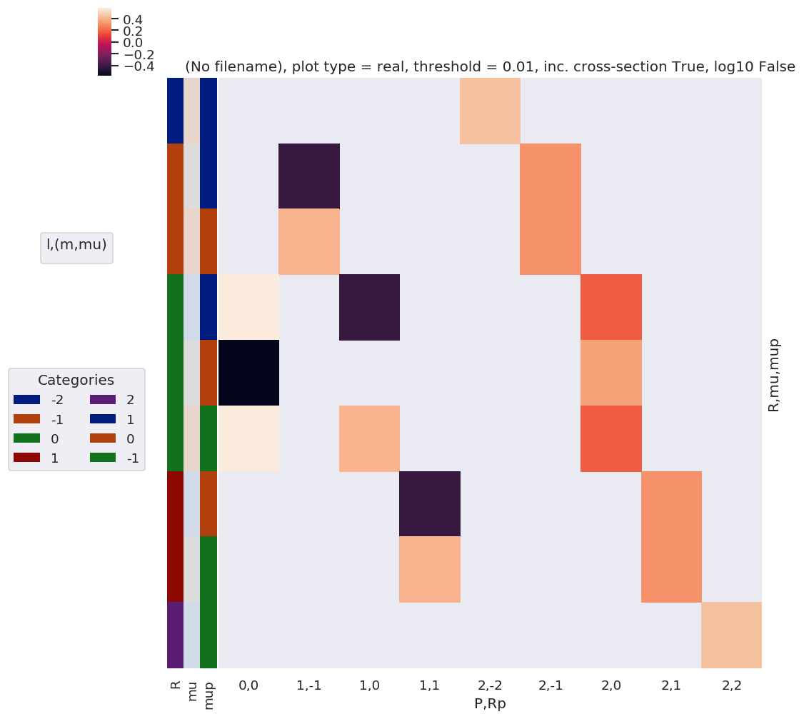
[29]:
# Plot
xDim = {'PRp':['P','Rp']}
# daPlot, daPlotpd, legendList, gFig = ep.lmPlot(testMult, plotDims=plotDimsRed, xDim=xDim, pType = 'r')
daPlot, daPlotpd, legendList, gFig = ep.lmPlot(lambdaTermResort, xDim=xDim, pType = 'r')
daPlotpd
Plotting data (No filename), pType=r, thres=0.01, with Seaborn
No handles with labels found to put in legend.
[29]:
| P | 0 | 1 | 2 | ||||||||
|---|---|---|---|---|---|---|---|---|---|---|---|
| Rp | 0 | -1 | 0 | 1 | -2 | -1 | 0 | 1 | 2 | ||
| R | mu | mup | |||||||||
| -2 | 1 | 1 | NaN | NaN | NaN | NaN | 0.447214 | NaN | NaN | NaN | NaN |
| -1 | 0 | 1 | NaN | -0.408248 | NaN | NaN | NaN | 0.316228 | NaN | NaN | NaN |
| 1 | 0 | NaN | 0.408248 | NaN | NaN | NaN | 0.316228 | NaN | NaN | NaN | |
| 0 | -1 | 1 | 0.57735 | NaN | -0.408248 | NaN | NaN | NaN | 0.182574 | NaN | NaN |
| 0 | 0 | -0.57735 | NaN | NaN | NaN | NaN | NaN | 0.365148 | NaN | NaN | |
| 1 | -1 | 0.57735 | NaN | 0.408248 | NaN | NaN | NaN | 0.182574 | NaN | NaN | |
| 1 | -1 | 0 | NaN | NaN | NaN | -0.408248 | NaN | NaN | NaN | 0.316228 | NaN |
| 0 | -1 | NaN | NaN | NaN | 0.408248 | NaN | NaN | NaN | 0.316228 | NaN | |
| 2 | -1 | -1 | NaN | NaN | NaN | NaN | NaN | NaN | NaN | NaN | 0.447214 |
Check component terms are as expected
Should have R = Rp for z case, and wD terms = 1 or 0.
[30]:
lambdaTablepd, _ = ep.util.multiDimXrToPD(lambdaTable, colDims=xDim, dropna=True)
lambdaTablepd
[30]:
| P | 0 | 1 | 2 | ||||||||||
|---|---|---|---|---|---|---|---|---|---|---|---|---|---|
| Rp | 0 | -1 | 0 | 1 | -2 | -1 | 0 | 1 | 2 | ||||
| R | l | lp | mu | mup | |||||||||
| -2 | 1 | 1 | -1 | -1 | NaN | NaN | NaN | NaN | NaN | NaN | NaN | NaN | 0.447214 |
| 0 | NaN | NaN | NaN | NaN | NaN | NaN | NaN | -0.316228 | NaN | ||||
| 1 | NaN | NaN | NaN | NaN | NaN | NaN | 0.182574 | NaN | NaN | ||||
| 0 | -1 | NaN | NaN | NaN | NaN | NaN | NaN | NaN | -0.316228 | NaN | |||
| 0 | NaN | NaN | NaN | NaN | NaN | NaN | 0.365148 | NaN | NaN | ||||
| 1 | NaN | NaN | NaN | NaN | NaN | -0.316228 | NaN | NaN | NaN | ||||
| 1 | -1 | NaN | NaN | NaN | NaN | NaN | NaN | 0.182574 | NaN | NaN | |||
| 0 | NaN | NaN | NaN | NaN | NaN | -0.316228 | NaN | NaN | NaN | ||||
| 1 | NaN | NaN | NaN | NaN | 0.447214 | NaN | NaN | NaN | NaN | ||||
| -1 | 1 | 1 | -1 | -1 | NaN | NaN | NaN | NaN | NaN | NaN | NaN | NaN | 0.447214 |
| 0 | NaN | NaN | NaN | 0.408248 | NaN | NaN | NaN | -0.316228 | NaN | ||||
| 1 | NaN | NaN | -0.408248 | NaN | NaN | NaN | 0.182574 | NaN | NaN | ||||
| 0 | -1 | NaN | NaN | NaN | -0.408248 | NaN | NaN | NaN | -0.316228 | NaN | |||
| 0 | NaN | NaN | NaN | NaN | NaN | NaN | 0.365148 | NaN | NaN | ||||
| 1 | NaN | 0.408248 | NaN | NaN | NaN | -0.316228 | NaN | NaN | NaN | ||||
| 1 | -1 | NaN | NaN | 0.408248 | NaN | NaN | NaN | 0.182574 | NaN | NaN | |||
| 0 | NaN | -0.408248 | NaN | NaN | NaN | -0.316228 | NaN | NaN | NaN | ||||
| 1 | NaN | NaN | NaN | NaN | 0.447214 | NaN | NaN | NaN | NaN | ||||
| 0 | 1 | 1 | -1 | -1 | NaN | NaN | NaN | NaN | NaN | NaN | NaN | NaN | 0.447214 |
| 0 | NaN | NaN | NaN | 0.408248 | NaN | NaN | NaN | -0.316228 | NaN | ||||
| 1 | 0.57735 | NaN | -0.408248 | NaN | NaN | NaN | 0.182574 | NaN | NaN | ||||
| 0 | -1 | NaN | NaN | NaN | -0.408248 | NaN | NaN | NaN | -0.316228 | NaN | |||
| 0 | -0.57735 | NaN | NaN | NaN | NaN | NaN | 0.365148 | NaN | NaN | ||||
| 1 | NaN | 0.408248 | NaN | NaN | NaN | -0.316228 | NaN | NaN | NaN | ||||
| 1 | -1 | 0.57735 | NaN | 0.408248 | NaN | NaN | NaN | 0.182574 | NaN | NaN | |||
| 0 | NaN | -0.408248 | NaN | NaN | NaN | -0.316228 | NaN | NaN | NaN | ||||
| 1 | NaN | NaN | NaN | NaN | 0.447214 | NaN | NaN | NaN | NaN | ||||
| 1 | 1 | 1 | -1 | -1 | NaN | NaN | NaN | NaN | NaN | NaN | NaN | NaN | 0.447214 |
| 0 | NaN | NaN | NaN | 0.408248 | NaN | NaN | NaN | -0.316228 | NaN | ||||
| 1 | NaN | NaN | -0.408248 | NaN | NaN | NaN | 0.182574 | NaN | NaN | ||||
| 0 | -1 | NaN | NaN | NaN | -0.408248 | NaN | NaN | NaN | -0.316228 | NaN | |||
| 0 | NaN | NaN | NaN | NaN | NaN | NaN | 0.365148 | NaN | NaN | ||||
| 1 | NaN | 0.408248 | NaN | NaN | NaN | -0.316228 | NaN | NaN | NaN | ||||
| 1 | -1 | NaN | NaN | 0.408248 | NaN | NaN | NaN | 0.182574 | NaN | NaN | |||
| 0 | NaN | -0.408248 | NaN | NaN | NaN | -0.316228 | NaN | NaN | NaN | ||||
| 1 | NaN | NaN | NaN | NaN | 0.447214 | NaN | NaN | NaN | NaN | ||||
| 2 | 1 | 1 | -1 | -1 | NaN | NaN | NaN | NaN | NaN | NaN | NaN | NaN | 0.447214 |
| 0 | NaN | NaN | NaN | NaN | NaN | NaN | NaN | -0.316228 | NaN | ||||
| 1 | NaN | NaN | NaN | NaN | NaN | NaN | 0.182574 | NaN | NaN | ||||
| 0 | -1 | NaN | NaN | NaN | NaN | NaN | NaN | NaN | -0.316228 | NaN | |||
| 0 | NaN | NaN | NaN | NaN | NaN | NaN | 0.365148 | NaN | NaN | ||||
| 1 | NaN | NaN | NaN | NaN | NaN | -0.316228 | NaN | NaN | NaN | ||||
| 1 | -1 | NaN | NaN | NaN | NaN | NaN | NaN | 0.182574 | NaN | NaN | |||
| 0 | NaN | NaN | NaN | NaN | NaN | -0.316228 | NaN | NaN | NaN | ||||
| 1 | NaN | NaN | NaN | NaN | 0.447214 | NaN | NaN | NaN | NaN | ||||
[31]:
lambdaTermResortpd, _ = ep.util.multiDimXrToPD(lambdaTermResort, colDims=xDim, dropna=True)
lambdaTermResortpd

# Think this is as per lambdaTable terms, just different ordering - because lambdaTable doesn't include some phase switches?
[31]:
| P | 0 | 1 | 2 | ||||||||
|---|---|---|---|---|---|---|---|---|---|---|---|
| Rp | 0 | -1 | 0 | 1 | -2 | -1 | 0 | 1 | 2 | ||
| R | mu | mup | |||||||||
| -2 | -1 | -1 | NaN | NaN | NaN | NaN | NaN | NaN | NaN | NaN | 0.000000+0.000000j |
| 0 | NaN | NaN | NaN | NaN | NaN | NaN | NaN | 0.000000+0.000000j | NaN | ||
| 1 | NaN | NaN | NaN | NaN | NaN | NaN | 0.000000+0.000000j | NaN | NaN | ||
| 0 | -1 | NaN | NaN | NaN | NaN | NaN | NaN | NaN | 0.000000+0.000000j | NaN | |
| 0 | NaN | NaN | NaN | NaN | NaN | NaN | 0.000000+0.000000j | NaN | NaN | ||
| 1 | NaN | NaN | NaN | NaN | NaN | 0.000000+0.000000j | NaN | NaN | NaN | ||
| 1 | -1 | NaN | NaN | NaN | NaN | NaN | NaN | 0.000000+0.000000j | NaN | NaN | |
| 0 | NaN | NaN | NaN | NaN | NaN | 0.000000+0.000000j | NaN | NaN | NaN | ||
| 1 | NaN | NaN | NaN | NaN | 0.447214+0.000000j | NaN | NaN | NaN | NaN | ||
| -1 | -1 | -1 | NaN | NaN | NaN | NaN | NaN | NaN | NaN | NaN | 0.000000+0.000000j |
| 0 | NaN | NaN | NaN | 0.000000+0.000000j | NaN | NaN | NaN | 0.000000+0.000000j | NaN | ||
| 1 | NaN | NaN | 0.000000+0.000000j | NaN | NaN | NaN | 0.000000+0.000000j | NaN | NaN | ||
| 0 | -1 | NaN | NaN | NaN | 0.000000+0.000000j | NaN | NaN | NaN | 0.000000+0.000000j | NaN | |
| 0 | NaN | NaN | NaN | NaN | NaN | NaN | 0.000000+0.000000j | NaN | NaN | ||
| 1 | NaN | -0.408248+0.000000j | NaN | NaN | NaN | 0.316228+0.000000j | NaN | NaN | NaN | ||
| 1 | -1 | NaN | NaN | 0.000000+0.000000j | NaN | NaN | NaN | 0.000000+0.000000j | NaN | NaN | |
| 0 | NaN | 0.408248+0.000000j | NaN | NaN | NaN | 0.316228+0.000000j | NaN | NaN | NaN | ||
| 1 | NaN | NaN | NaN | NaN | 0.000000+0.000000j | NaN | NaN | NaN | NaN | ||
| 0 | -1 | -1 | NaN | NaN | NaN | NaN | NaN | NaN | NaN | NaN | 0.000000+0.000000j |
| 0 | NaN | NaN | NaN | 0.000000+0.000000j | NaN | NaN | NaN | 0.000000+0.000000j | NaN | ||
| 1 | 0.577350+0.000000j | NaN | -0.408248+0.000000j | NaN | NaN | NaN | 0.182574+0.000000j | NaN | NaN | ||
| 0 | -1 | NaN | NaN | NaN | 0.000000+0.000000j | NaN | NaN | NaN | 0.000000+0.000000j | NaN | |
| 0 | -0.577350+0.000000j | NaN | NaN | NaN | NaN | NaN | 0.365148+0.000000j | NaN | NaN | ||
| 1 | NaN | 0.000000+0.000000j | NaN | NaN | NaN | 0.000000+0.000000j | NaN | NaN | NaN | ||
| 1 | -1 | 0.577350+0.000000j | NaN | 0.408248+0.000000j | NaN | NaN | NaN | 0.182574+0.000000j | NaN | NaN | |
| 0 | NaN | 0.000000+0.000000j | NaN | NaN | NaN | 0.000000+0.000000j | NaN | NaN | NaN | ||
| 1 | NaN | NaN | NaN | NaN | 0.000000+0.000000j | NaN | NaN | NaN | NaN | ||
| 1 | -1 | -1 | NaN | NaN | NaN | NaN | NaN | NaN | NaN | NaN | 0.000000+0.000000j |
| 0 | NaN | NaN | NaN | -0.408248+0.000000j | NaN | NaN | NaN | 0.316228+0.000000j | NaN | ||
| 1 | NaN | NaN | 0.000000+0.000000j | NaN | NaN | NaN | 0.000000+0.000000j | NaN | NaN | ||
| 0 | -1 | NaN | NaN | NaN | 0.408248+0.000000j | NaN | NaN | NaN | 0.316228+0.000000j | NaN | |
| 0 | NaN | NaN | NaN | NaN | NaN | NaN | 0.000000+0.000000j | NaN | NaN | ||
| 1 | NaN | 0.000000+0.000000j | NaN | NaN | NaN | 0.000000+0.000000j | NaN | NaN | NaN | ||
| 1 | -1 | NaN | NaN | 0.000000+0.000000j | NaN | NaN | NaN | 0.000000+0.000000j | NaN | NaN | |
| 0 | NaN | 0.000000+0.000000j | NaN | NaN | NaN | 0.000000+0.000000j | NaN | NaN | NaN | ||
| 1 | NaN | NaN | NaN | NaN | 0.000000+0.000000j | NaN | NaN | NaN | NaN | ||
| 2 | -1 | -1 | NaN | NaN | NaN | NaN | NaN | NaN | NaN | NaN | 0.447214+0.000000j |
| 0 | NaN | NaN | NaN | NaN | NaN | NaN | NaN | 0.000000+0.000000j | NaN | ||
| 1 | NaN | NaN | NaN | NaN | NaN | NaN | 0.000000+0.000000j | NaN | NaN | ||
| 0 | -1 | NaN | NaN | NaN | NaN | NaN | NaN | NaN | 0.000000+0.000000j | NaN | |
| 0 | NaN | NaN | NaN | NaN | NaN | NaN | 0.000000+0.000000j | NaN | NaN | ||
| 1 | NaN | NaN | NaN | NaN | NaN | 0.000000+0.000000j | NaN | NaN | NaN | ||
| 1 | -1 | NaN | NaN | NaN | NaN | NaN | NaN | 0.000000+0.000000j | NaN | NaN | |
| 0 | NaN | NaN | NaN | NaN | NaN | 0.000000+0.000000j | NaN | NaN | NaN | ||
| 1 | NaN | NaN | NaN | NaN | 0.000000+0.000000j | NaN | NaN | NaN | NaN | ||
[32]:
# wigner D term looks good.
lambdaDpd, _ = ep.util.multiDimXrToPD(lambdaD.sel({'Labels':'z'}), colDims=xDim, dropna=True)
lambdaDpd
[32]:
| P | 0 | 1 | 2 | ||||||||||||
|---|---|---|---|---|---|---|---|---|---|---|---|---|---|---|---|
| Rp | 2 | 1 | 0 | -1 | -2 | 2 | 1 | 0 | -1 | -2 | 2 | 1 | 0 | -1 | -2 |
| R | |||||||||||||||
| 2 | NaN | NaN | NaN | NaN | NaN | NaN | NaN | NaN | NaN | NaN | 1.000000-0.000000j | 0.000000-0.000000j | 0.000000-0.000000j | 0.000000-0.000000j | 0.000000-0.000000j |
| 1 | NaN | NaN | NaN | NaN | NaN | 0.000000-0.000000j | 1.000000-0.000000j | 0.000000-0.000000j | 0.000000-0.000000j | 0.000000-0.000000j | 0.000000-0.000000j | 1.000000-0.000000j | 0.000000-0.000000j | 0.000000-0.000000j | 0.000000-0.000000j |
| 0 | 0.000000-0.000000j | 0.000000-0.000000j | 1.000000-0.000000j | 0.000000-0.000000j | 0.000000-0.000000j | 0.000000-0.000000j | 0.000000-0.000000j | 1.000000-0.000000j | 0.000000-0.000000j | 0.000000-0.000000j | 0.000000-0.000000j | 0.000000-0.000000j | 1.000000-0.000000j | 0.000000-0.000000j | 0.000000-0.000000j |
| -1 | NaN | NaN | NaN | NaN | NaN | 0.000000-0.000000j | 0.000000-0.000000j | 0.000000-0.000000j | 1.000000+0.000000j | 0.000000-0.000000j | 0.000000-0.000000j | 0.000000-0.000000j | 0.000000-0.000000j | 1.000000+0.000000j | 0.000000-0.000000j |
| -2 | NaN | NaN | NaN | NaN | NaN | NaN | NaN | NaN | NaN | NaN | 0.000000-0.000000j | 0.000000-0.000000j | 0.000000-0.000000j | 0.000000-0.000000j | 1.000000+0.000000j |
Build full calculation from functions
Use mfblmGeom.py as template: basically just need modified lambda term as above, and new alignment term, and rest of calculation should be identical.
[33]:
# Check polProd term - incorporate alignment term here...?

# Existing terms
# polProd = (EPRXresort * lambdaTermResort)

# sumDimsPol = ['P','R','Rp','p']
# polProd = polProd.sum(sumDimsPol)

# Test with alignment term
polProd = (EPRXresort * lambdaTermResort * AFterm)
sumDimsPol = ['P','R','Rp','p', 'S-Rp']
polProd = polProd.sum(sumDimsPol)
# Looks OK - keeps correct dims in test case! 270 terms.
NOW implemented in ep.geomFunc.afblmGeom.py
Testing…
16/06/20
Test code adapted from previous round of AF tests, http://localhost:8888/lab/tree/dev/ePSproc/ePSproc_AFBLM_calcs_bench_100220.ipynb
See also MFBLM test code, http://localhost:8888/lab/tree/dev/ePSproc/geometric_method_dev_2020/geometric_method_dev_pt2_170320_v090620.ipynb
Load data
[34]:
# Load data from modPath\data
dataPath = os.path.join(modPath, 'data', 'photoionization')
dataFile = os.path.join(dataPath, 'n2_3sg_0.1-50.1eV_A2.inp.out')  # Set for sample N2 data for testing

# Scan data file
dataSet = ep.readMatEle(fileIn = dataFile)
dataXS = ep.readMatEle(fileIn = dataFile, recordType = 'CrossSection')  # XS info currently not set in NO2 sample file.
*** ePSproc readMatEle(): scanning files for DumpIdy segments.

*** Scanning file(s)
['D:\\code\\github\\ePSproc\\data\\photoionization\\n2_3sg_0.1-50.1eV_A2.inp.out']

*** Reading ePS output file:  D:\code\github\ePSproc\data\photoionization\n2_3sg_0.1-50.1eV_A2.inp.out
Expecting 51 energy points.
Expecting 2 symmetries.
Scanning CrossSection segments.
Expecting 102 DumpIdy segments.
Found 102 dumpIdy segments (sets of matrix elements).

Processing segments to Xarrays...
Processed 102 sets of DumpIdy file segments, (0 blank)
*** ePSproc readMatEle(): scanning files for CrossSection segments.

*** Scanning file(s)
['D:\\code\\github\\ePSproc\\data\\photoionization\\n2_3sg_0.1-50.1eV_A2.inp.out']

*** Reading ePS output file:  D:\code\github\ePSproc\data\photoionization\n2_3sg_0.1-50.1eV_A2.inp.out
Expecting 51 energy points.
Expecting 2 symmetries.
Scanning CrossSection segments.
Expecting 3 CrossSection segments.
Found 3 CrossSection segments (sets of results).
Processed 3 sets of CrossSection file segments, (0 blank)
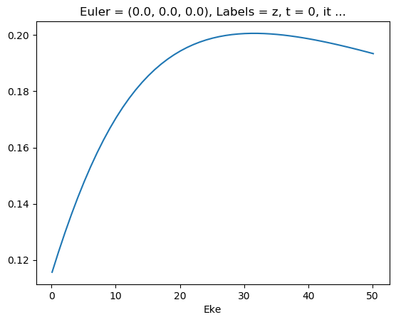
Plot ePS results (isotropic case)
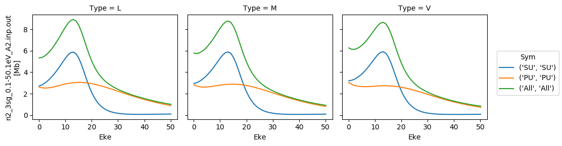
[35]:
# Plot cross sections using Xarray functionality
# Set here to plot per file - should add some logic to combine files.
for data in dataXS:
    daPlot = data.sel(XC='SIGMA')
    daPlot.plot.line(x='Eke', col='Type')
[35]:
<xarray.plot.facetgrid.FacetGrid at 0x2c402402630>
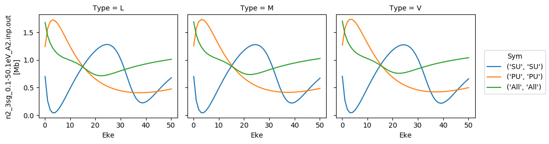
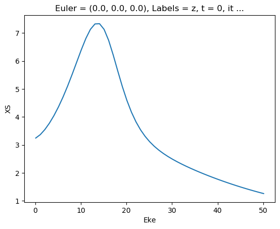
[36]:
# Repeat for betas
for data in dataXS:
    daPlot = data.sel(XC='BETA')
    daPlot.plot.line(x='Eke', col='Type')
[36]:
<xarray.plot.facetgrid.FacetGrid at 0x2c402584828>
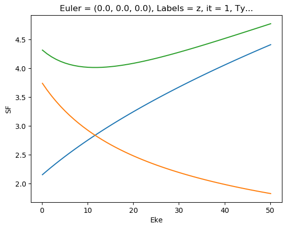
Try new AF calculation - isotropic (default) case
[37]:
# Tabulate & plot matrix elements vs. Eke
selDims = {'it':1, 'Type':'L'}
matE = dataSet[0].sel(selDims)  # Set for N2 case, length-gauge results only.
daPlot, daPlotpd, legendList, gFig = ep.lmPlot(matE, xDim = 'Eke', pType = 'r', fillna = True)
daPlotpd
Plotting data n2_3sg_0.1-50.1eV_A2.inp.out, pType=r, thres=0.01, with Seaborn
[37]:
| Eke | 0.1 | 1.1 | 2.1 | 3.1 | 4.1 | 5.1 | 6.1 | 7.1 | 8.1 | 9.1 | ... | 41.1 | 42.1 | 43.1 | 44.1 | 45.1 | 46.1 | 47.1 | 48.1 | 49.1 | 50.1 | |||||
|---|---|---|---|---|---|---|---|---|---|---|---|---|---|---|---|---|---|---|---|---|---|---|---|---|---|---|
| Cont | Targ | Total | l | m | mu | |||||||||||||||||||||
| PU | SG | PU | 1 | -1 | 1 | -6.203556 | 7.496908 | 3.926892 | 1.071093 | -0.335132 | -1.043391 | -1.396885 | -1.554984 | -1.598812 | -1.573327 | ... | -0.396306 | -0.422225 | -0.448003 | -0.473466 | -0.498463 | -0.522867 | -0.546573 | -0.569493 | -0.591558 | -0.612712 |
| 1 | -1 | -6.203556 | 7.496908 | 3.926892 | 1.071093 | -0.335132 | -1.043391 | -1.396885 | -1.554984 | -1.598812 | -1.573327 | ... | -0.396306 | -0.422225 | -0.448003 | -0.473466 | -0.498463 | -0.522867 | -0.546573 | -0.569493 | -0.591558 | -0.612712 | ||||
| 3 | -1 | 1 | -2.090641 | -1.723467 | -3.571018 | -1.703191 | 0.232612 | 1.862713 | 3.201022 | 4.298839 | 5.198215 | 5.929303 | ... | 1.200463 | 1.040074 | 0.892501 | 0.757189 | 0.633556 | 0.521004 | 0.418928 | 0.326726 | 0.243800 | 0.169566 | |||
| 1 | -1 | -2.090641 | -1.723467 | -3.571018 | -1.703191 | 0.232612 | 1.862713 | 3.201022 | 4.298839 | 5.198215 | 5.929303 | ... | 1.200463 | 1.040074 | 0.892501 | 0.757189 | 0.633556 | 0.521004 | 0.418928 | 0.326726 | 0.243800 | 0.169566 | ||||
| 5 | -1 | 1 | 0.000000 | 0.013246 | 0.000000 | -0.013096 | -0.024367 | -0.033455 | -0.042762 | -0.053765 | -0.067354 | -0.083946 | ... | -0.325544 | -0.318791 | -0.312332 | -0.306211 | -0.300456 | -0.295091 | -0.290130 | -0.285584 | -0.281453 | -0.277737 | |||
| 1 | -1 | 0.000000 | 0.013246 | 0.000000 | -0.013096 | -0.024367 | -0.033455 | -0.042762 | -0.053765 | -0.067354 | -0.083946 | ... | -0.325544 | -0.318791 | -0.312332 | -0.306211 | -0.300456 | -0.295091 | -0.290130 | -0.285584 | -0.281453 | -0.277737 | ||||
| 7 | -1 | 1 | 0.000000 | 0.000000 | 0.000000 | 0.000000 | 0.000000 | 0.000000 | 0.000000 | 0.000000 | 0.000000 | 0.000000 | ... | 0.027469 | 0.028083 | 0.028678 | 0.029257 | 0.029823 | 0.030377 | 0.030923 | 0.031461 | 0.031994 | 0.032523 | |||
| 1 | -1 | 0.000000 | 0.000000 | 0.000000 | 0.000000 | 0.000000 | 0.000000 | 0.000000 | 0.000000 | 0.000000 | 0.000000 | ... | 0.027469 | 0.028083 | 0.028678 | 0.029257 | 0.029823 | 0.030377 | 0.030923 | 0.031461 | 0.031994 | 0.032523 | ||||
| SU | SG | SU | 1 | 0 | 0 | 6.246520 | -10.081763 | -8.912214 | -5.342049 | -3.160539 | -1.795783 | -0.867993 | -0.174154 | 0.400643 | 0.926420 | ... | -0.854886 | -0.940017 | -1.021577 | -1.099776 | -1.174787 | -1.246759 | -1.315814 | -1.382058 | -1.445582 | -1.506467 |
| 3 | 0 | 0 | 2.605768 | 2.775108 | 4.733473 | 1.677812 | -1.450830 | -4.187395 | -6.554491 | -8.601759 | -10.343109 | -11.747922 | ... | -0.293053 | -0.441416 | -0.579578 | -0.708075 | -0.827415 | -0.938075 | -1.040506 | -1.135134 | -1.222361 | -1.302566 | |||
| 5 | 0 | 0 | 0.000000 | -0.020864 | 0.000000 | 0.024263 | 0.042694 | 0.059142 | 0.077308 | 0.099330 | 0.126227 | 0.157745 | ... | 0.490499 | 0.511546 | 0.531810 | 0.551281 | 0.569951 | 0.587815 | 0.604868 | 0.621107 | 0.636528 | 0.651132 | |||
| 7 | 0 | 0 | 0.000000 | 0.000000 | 0.000000 | 0.000000 | 0.000000 | 0.000000 | 0.000000 | 0.000000 | 0.000000 | 0.000000 | ... | -0.039566 | -0.041422 | -0.043265 | -0.045092 | -0.046901 | -0.048689 | -0.050453 | -0.052190 | -0.053899 | -0.055577 |
12 rows × 51 columns
[38]:
phaseConvention = 'E'  # Set phase conventions used in the numerics - for ePolyScat matrix elements, set to 'E', to match defns. above.

symSum = False  # Sum over symmetry groups, or keep separate?
SFflag = True  # Include scaling factor to Mb in calculation?
thres = 1e-4
RX = ep.setPolGeoms()  # Set default pol geoms (z,x,y), or will be set by mfblmXprod() defaults - FOR AF case this is only used to set 'z' geom for unity wigner D's - should rationalise this!

start = time.time()
mTermST, mTermS, mTermTest = ep.geomFunc.afblmXprod(dataSet[0], QNs = None, RX=RX, thres = thres, selDims = {'it':1, 'Type':'L'}, thresDims='Eke', symSum=symSum, SFflag=True, phaseConvention=phaseConvention)
end = time.time()
print('Elapsed time = {0} seconds, for {1} energy points, {2} polarizations, threshold={3}.'.format((end-start), mTermST.Eke.size, RX.size, thres))

# Elapsed time = 3.3885273933410645 seconds, for 51 energy points, 3 polarizations, threshold=0.01.
# Elapsed time = 5.059587478637695 seconds, for 51 energy points, 3 polarizations, threshold=0.0001.
Elapsed time = 2.529463768005371 seconds, for 51 energy points, 3 polarizations, threshold=0.0001.
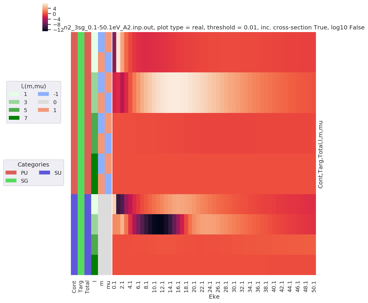
[39]:
# Full results (before summation)
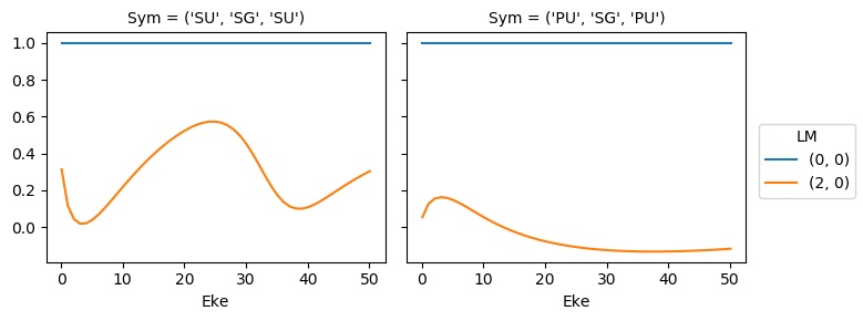
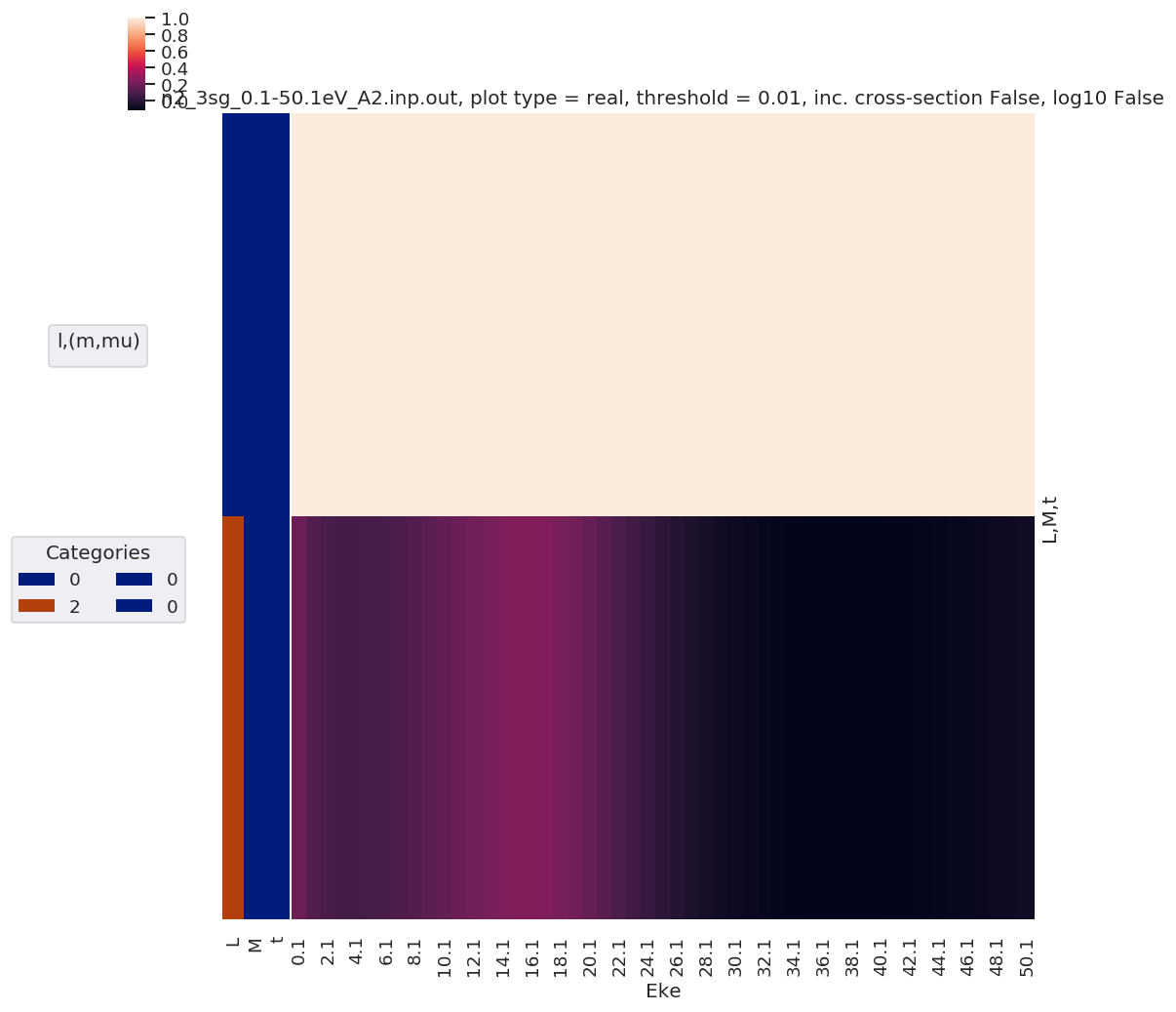
mTermST.attrs['dataType'] = 'matE' # Set matE here to allow for correct plotting of sym dims.
plotDimsRed = ['Labels','L','M'] # Set plotDims to fix dim ordering in plot
if not symSum:
plotDimsRed.extend(['Cont','Targ','Total'])
daPlot, daPlotpd, legendList, gFig = ep.lmPlot(mTermST, plotDims=plotDimsRed, xDim='Eke', sumDims=None, pType = 'r', thres = 0.01, fillna = True, SFflag=False)
# daPlot, daPlotpd, legendList, gFig = ep.lmPlot(mTermST, xDim='Eke', sumDims=None, pType = 'r', thres = 0.01, fillna = True) # If plotDims is not passed use default ordering.
Plotting data n2_3sg_0.1-50.1eV_A2.inp.out, pType=r, thres=0.01, with Seaborn
No handles with labels found to put in legend.
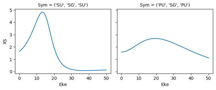
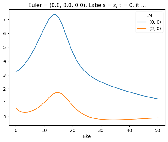
[40]:
mTermST.XS.real.squeeze().plot.line(x='Eke', col='Sym');
ep.util.matEleSelector(mTermST, thres = 0.1, dims='Eke').real.squeeze().plot.line(x='Eke', col='Sym');
Try sym summation…
[41]:
phaseConvention = 'E'  # Set phase conventions used in the numerics - for ePolyScat matrix elements, set to 'E', to match defns. above.

symSum = True  # Sum over symmetry groups, or keep separate?
SFflag = True  # Include scaling factor to Mb in calculation?
thres = 1e-4
RX = ep.setPolGeoms()  # Set default pol geoms (z,x,y), or will be set by mfblmXprod() defaults - FOR AF case this is only used to set 'z' geom for unity wigner D's - should rationalise this!

start = time.time()
mTermST, mTermS, mTermTest = ep.geomFunc.afblmXprod(dataSet[0], QNs = None, RX=RX, thres = thres, selDims = {'it':1, 'Type':'L'}, thresDims='Eke', symSum=symSum, SFflag=SFflag, phaseConvention=phaseConvention)
end = time.time()
print('Elapsed time = {0} seconds, for {1} energy points, {2} polarizations, threshold={3}.'.format((end-start), mTermST.Eke.size, RX.size, thres))

# Elapsed time = 3.3885273933410645 seconds, for 51 energy points, 3 polarizations, threshold=0.01.
# Elapsed time = 5.059587478637695 seconds, for 51 energy points, 3 polarizations, threshold=0.0001.
Elapsed time = 2.300682306289673 seconds, for 51 energy points, 3 polarizations, threshold=0.0001.
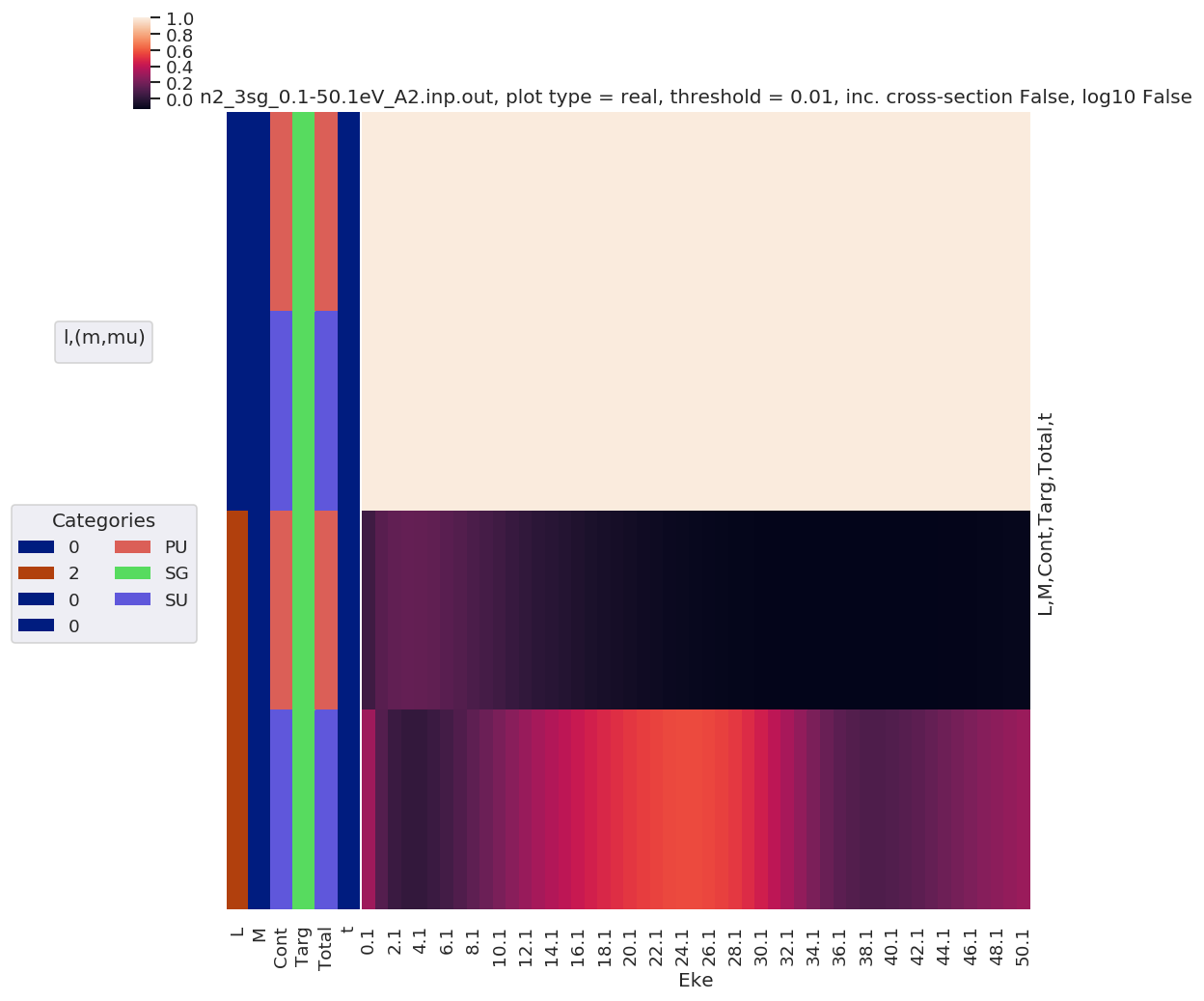
[42]:
# Full results (before summation)
mTermST.attrs['dataType'] = 'matE'  # Set matE here to allow for correct plotting of sym dims.

plotDimsRed = ['Labels','L','M']  # Set plotDims to fix dim ordering in plot
if not symSum:
    plotDimsRed.extend(['Cont','Targ','Total'])

daPlot, daPlotpd, legendList, gFig = ep.lmPlot(mTermST, plotDims=plotDimsRed, xDim='Eke', sumDims=None, pType = 'r', thres = 0.01, fillna = True, SFflag=False)

# daPlot, daPlotpd, legendList, gFig = ep.lmPlot(mTermST, xDim='Eke', sumDims=None, pType = 'r', thres = 0.01, fillna = True)  # If plotDims is not passed use default ordering.
Plotting data n2_3sg_0.1-50.1eV_A2.inp.out, pType=r, thres=0.01, with Seaborn
No handles with labels found to put in legend.
[43]:
mTermST.XS.real.squeeze().plot.line(x='Eke');

[44]:
ep.util.matEleSelector(mTermST, thres = 0.1, dims='Eke').real.squeeze().plot.line(x='Eke');
First attempt… with sym summation
- Looks quite different - might be SF issue with combining continua, and/or degen factor…?
- Looks same as previous AF code attempt (http://localhost:8888/lab/tree/dev/ePSproc/ePSproc_AFBLM_calcs_bench_100220.ipynb), suggesting something in degen/normalisation in formalism amiss?
[45]:
# ep.util.matEleSelector(mTermST, thres = 0.1, dims='Eke').real.squeeze().plot.line(x='Eke');
ep.util.matEleSelector(mTermST, thres = 0.1, dims='Eke').imag.squeeze().plot.line(x='Eke');
Test mult and renorm - seems like E-dependent XS issue here…
[ ]:
[46]:
mTermTest = mTermST.copy()
# mTermTest.values = mTermTest*mTermTest.SF
# mTermTest.values = mTermTest/mTermTest.SF.pipe(np.abs)
mTermTest.values = mTermTest/mTermTest.SF
ep.util.matEleSelector(mTermTest, thres = 0.1, dims='Eke').real.squeeze().plot.line(x='Eke');
[47]:
ep.util.matEleSelector(mTermST['XS'], thres = 0.1, dims='Eke').real.squeeze().plot.line(x='Eke');
[48]:
ep.util.matEleSelector(mTermST['SF'], thres = 0.1, dims='Eke').real.squeeze().plot.line(x='Eke');
ep.util.matEleSelector(mTermST['SF'], thres = 0.1, dims='Eke').imag.squeeze().plot.line(x='Eke');
ep.util.matEleSelector(mTermST['SF'], thres = 0.1, dims='Eke').pipe(np.abs).squeeze().plot.line(x='Eke');
[49]:
mTermST.values = mTermST*mTermST.XS
ep.util.matEleSelector(mTermST, thres = 0.1, dims='Eke').real.squeeze().plot.line(x='Eke');
[50]:
matE.values = matE * matE.SF
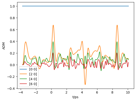
Test compared to experimental N2 AF results…
In this case MF PADs look good, so also expect good agreement with AF…
[51]:
# Adapted from ePSproc_AFBLM_testing_010519_300719.m
# Load ADMs for N2
from scipy.io import loadmat
ADMdataFile = os.path.join(modPath, 'data', 'alignment', 'N2_ADM_VM_290816.mat')
ADMs = loadmat(ADMdataFile)
[52]:
# Set tOffset for calcs, 3.76ps!!!
# This is because this is 2-pulse case, and will set t=0 to 2nd pulse (and matches defn. in N2 experimental paper)
tOffset = -3.76
ADMs['time'] = ADMs['time'] + tOffset
[53]:
# Plot
import matplotlib.pyplot as plt
plt.plot(ADMs['time'].T, np.real(ADMs['ADM'].T))
plt.legend(ADMs['ADMlist'])
plt.xlabel('t/ps')
plt.ylabel('ADM')
plt.show()
[53]:
[<matplotlib.lines.Line2D at 0x2c40580a0b8>,
 <matplotlib.lines.Line2D at 0x2c4007392e8>,
 <matplotlib.lines.Line2D at 0x2c400cc70f0>,
 <matplotlib.lines.Line2D at 0x2c400cc7f28>]
[53]:
<matplotlib.legend.Legend at 0x2c400960828>
[53]:
Text(0.5, 0, 't/ps')
[53]:
Text(0, 0.5, 'ADM')
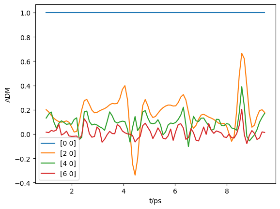
[54]:
# Selection & downsampling
trange=[1, 9.5]  # Set range in ps for calc
tStep=5  # Set tStep for downsampling

tMask = (ADMs['time']>trange[0]) * (ADMs['time']<trange[1])
ind = np.nonzero(tMask)[1][0::tStep]
At = ADMs['time'][:,ind].squeeze()
ADMin = ADMs['ADM'][:,ind]

print(f"Selecting {ind.size} points")

plt.plot(At, np.real(ADMin.T))
plt.legend(ADMs['ADMlist'])
plt.xlabel('t/ps')
plt.ylabel('ADM')
plt.show()

# Set in Xarray
ADMX = ep.setADMs(ADMs = ADMs['ADM'][:,ind], t=At, KQSLabels = ADMs['ADMlist'], addS = True)
# ADMX
Selecting 87 points
[54]:
[<matplotlib.lines.Line2D at 0x2c400b3b080>,
 <matplotlib.lines.Line2D at 0x2c4724dea20>,
 <matplotlib.lines.Line2D at 0x2c400b4f2e8>,
 <matplotlib.lines.Line2D at 0x2c400b4f208>]
[54]:
<matplotlib.legend.Legend at 0x2c4024c6908>
[54]:
Text(0.5, 0, 't/ps')
[54]:
Text(0, 0.5, 'ADM')
[73]:
# Run with sym summation...

phaseConvention = 'E'  # Set phase conventions used in the numerics - for ePolyScat matrix elements, set to 'E', to match defns. above.

symSum = True  # Sum over symmetry groups, or keep separate?
SFflag = False  # Include scaling factor to Mb in calculation?
BLMRenorm = False
thres = 1e-4
RX = ep.setPolGeoms()  # Set default pol geoms (z,x,y), or will be set by mfblmXprod() defaults - FOR AF case this is only used to set 'z' geom for unity wigner D's - should rationalise this!

start = time.time()
mTermST, mTermS, mTermTest = ep.geomFunc.afblmXprod(dataSet[0], QNs = None, AKQS=ADMX, RX=RX, thres = thres, selDims = {'it':1, 'Type':'L'}, thresDims='Eke',
                                                    symSum=symSum, SFflag=SFflag, BLMRenorm = BLMRenorm,
                                                    phaseConvention=phaseConvention)
end = time.time()
print('Elapsed time = {0} seconds, for {1} energy points, {2} polarizations, threshold={3}.'.format((end-start), mTermST.Eke.size, RX.size, thres))

# Elapsed time = 3.3885273933410645 seconds, for 51 energy points, 3 polarizations, threshold=0.01.
# Elapsed time = 5.059587478637695 seconds, for 51 energy points, 3 polarizations, threshold=0.0001.
Elapsed time = 3.8453733921051025 seconds, for 51 energy points, 3 polarizations, threshold=0.0001.
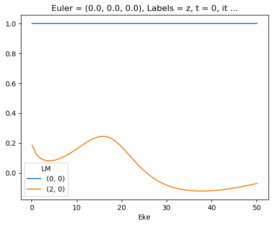
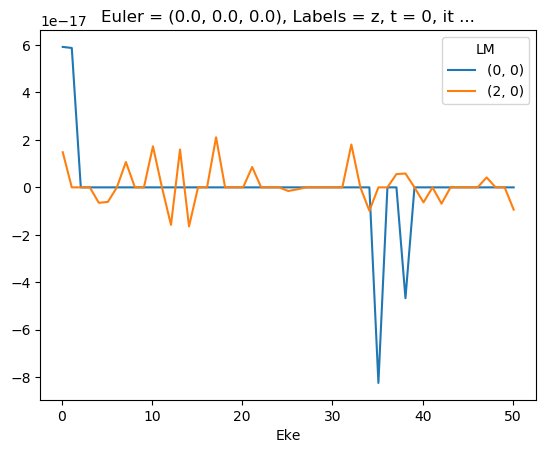
[74]:
# Full results (before summation)
mTermST.attrs['dataType'] = 'matE'  # Set matE here to allow for correct plotting of sym dims.

plotDimsRed = ['Labels','L','M']  # Set plotDims to fix dim ordering in plot
if not symSum:
    plotDimsRed.extend(['Cont','Targ','Total'])

# daPlot, daPlotpd, legendList, gFig = ep.lmPlot(mTermST, plotDims=plotDimsRed, xDim='Eke', sumDims=None, pType = 'r', thres = 0.01, fillna = True, SFflag=False)

# daPlot, daPlotpd, legendList, gFig = ep.lmPlot(mTermST, xDim='Eke', sumDims=None, pType = 'r', thres = 0.01, fillna = True)  # If plotDims is not passed use default ordering.
[75]:
# daPlot, daPlotpd, legendList, gFig = ep.lmPlot(mTermST.XS, plotDims=plotDimsRed, xDim='Eke', sumDims=None, pType = 'r', thres = 0.01, fillna = True, SFflag=False)
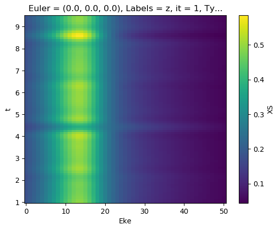
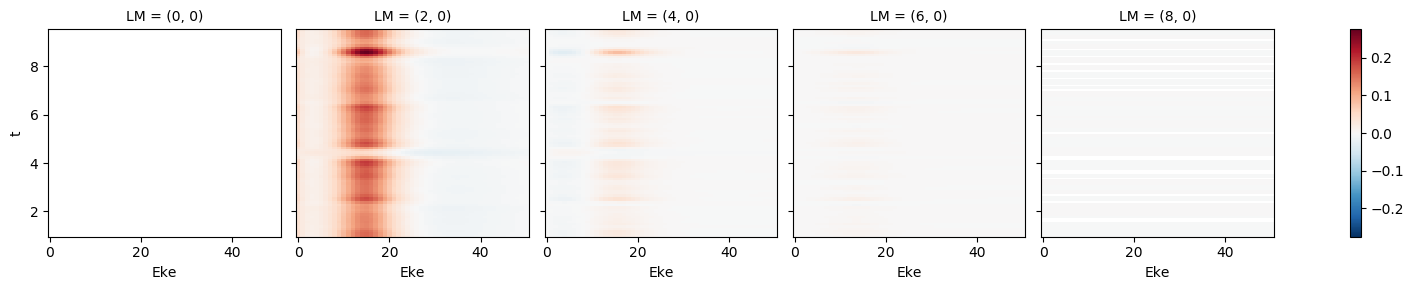
[76]:
mTermST.XS.real.plot()
mTermST.where(mTermST.L > 0).real.plot(col='LM')
[76]:
<matplotlib.collections.QuadMesh at 0x2c400c7a0b8>
[76]:
<xarray.plot.facetgrid.FacetGrid at 0x2c4058c19e8>
[77]:
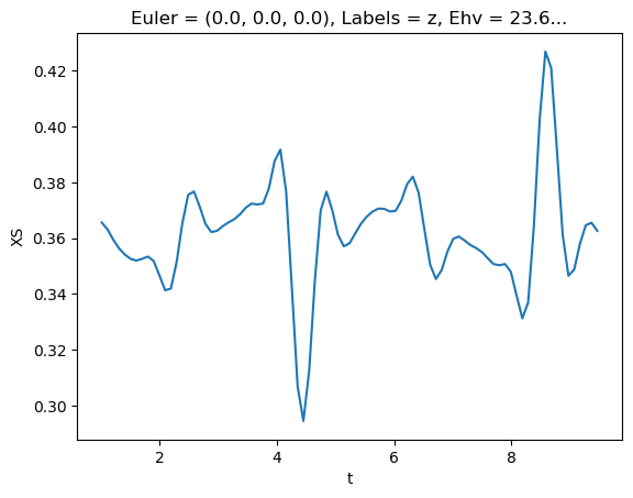
# Plot single energy XS
E = 8.1
mTermST.XS.sel({'Eke':E}).real.squeeze().plot.line(x='t');
[78]:
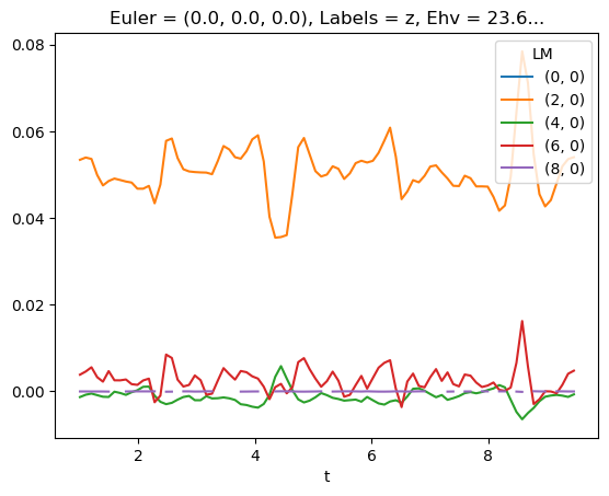
# LM with renorm
mTermST.sel({'Eke':E}).where(mTermST['L']>0).real.squeeze().plot.line(x='t');
[72]:
# LM * XS
# (mTermST * mTermST.XS).sel({'Eke':E}).where(mTermST['L']>0).real.squeeze().plot.line(x='t');
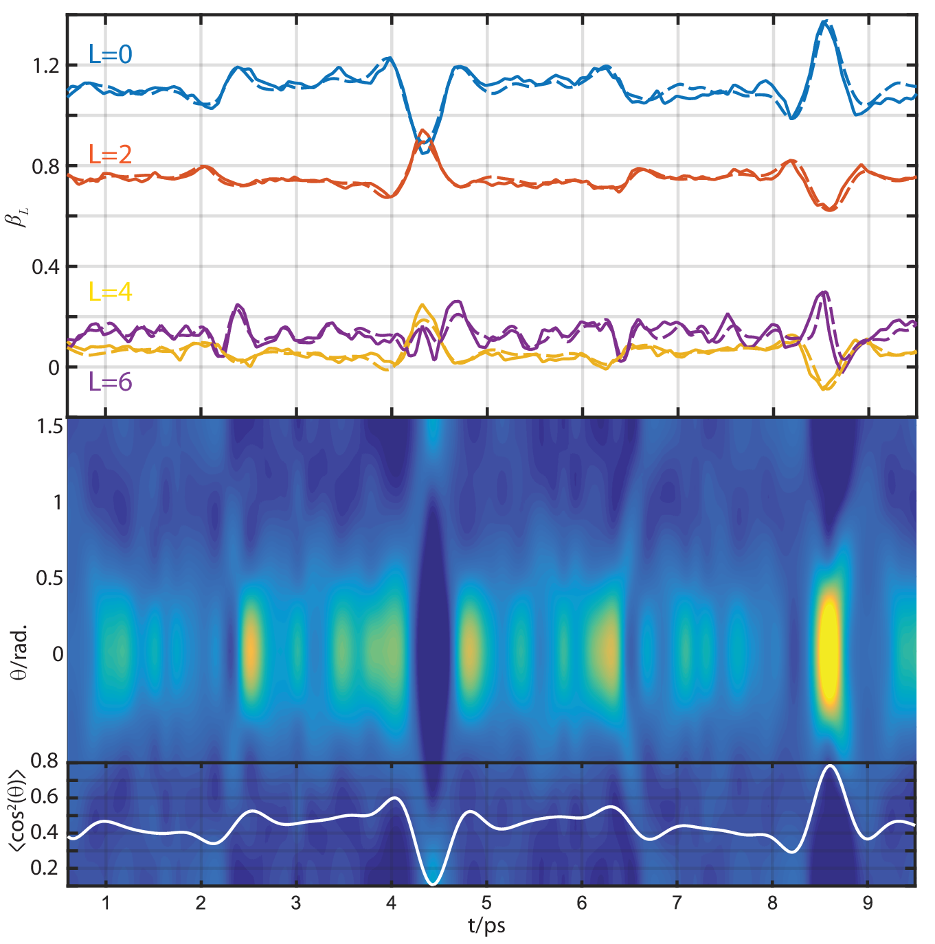
Experimental results
(Fig 2 from Marceau, Claude, Varun Makhija, Dominique Platzer, A. Yu. Naumov, P. B. Corkum, Albert Stolow, D. M. Villeneuve, and Paul Hockett. “Molecular Frame Reconstruction Using Time-Domain Photoionization Interferometry.” Physical Review Letters 119, no. 8 (August 2017): 083401. https://doi.org/10.1103/PhysRevLett.119.083401. Full data at https://doi.org/10.6084/m9.figshare.4480349.v10)
Currently:
- Relative signs/phases of betas look good at 4.1eV… but not at 7.1 or 8.1eV! (Experimental MFPAD comparison energy) - suggests still phase and/or renorm issue somewhere?
- Values still off, same issue probably.
- Might be phase issue with sum over rotation matrix elements, which are conj() in MF case, but not in original derivation here…? This could give 3j sign-flip, hence change calculated alignment response.
SCRATCH
[62]:
# Phase switch example
        if phaseCons['mfblmCons']['BLMmPhase']:
            QNsBLMtable[:,3] *= -1
            QNsBLMtable[:,5] *= -1
  File "<ipython-input-62-6783c300192b>", line 2
    if phaseCons['mfblmCons']['BLMmPhase']:
    ^
IndentationError: unexpected indent
[ ]:
def deltaKQS(QNs = None):
    phaseCons = setPhaseConventions(phaseConvention = phaseConvention)

    # If no QNs are passed, set for all possible terms
    if QNs is None:
        QNs = []

        # Set photon terms
        l = 1
        lp = 1

        # Loop to set all other QNs
        for mu in np.arange(-l, l+1):
            for mup in np.arange(-lp, lp+1):
                #for R in np.arange(-(l+lp)-1, l+lp+2):
                #    for P in np.arange(0, l+lp+1):
                for P in np.arange(0, l+lp+1):
                    # for Rp in np.arange(-P, P+1):  # Allow all Rp
                    # Rp = -(mu+mup)   # Fix Rp terms - not valid here, depends on other phase cons!
                    # for R in np.arange(-P, P+1):
                    #     # QNs.append([l, lp, P, mu, -mup, R, Rp])
                    #     if phaseCons['lambdaCons']['negRp']:
                    #         Rp *= -1
                    #     if phaseCons['lambdaCons']['negMup']:
                    #         QNs.append([l, lp, P, mu, -mup, Rp, R])   # 31/03/20: FIXED bug, (R,Rp) previously misordered!!!
                    #     else:
                    #         QNs.append([l, lp, P, mu, mup, Rp, R])

                    # Rearranged for specified Rp case
                    for R in np.arange(-P, P+1):
                        # if phaseCons['lambdaCons']['negMup']:
                        #     mup = -mup

                        if phaseCons['lambdaCons']['negRp']:
                            # Rp = mu+mup
                            Rp = mup - mu
                        else:
                            Rp = -(mu+mup)

                        # Switch mup sign for 3j?  To match old numerics, this is *after* Rp assignment (sigh).
                        if phaseCons['lambdaCons']['negMup']:
                            mup = -mup

                        QNs.append([l, lp, P, mu, mup, Rp, R])

        QNs = np.array(QNs)