Frame definitions
14/03/24
Canonical frame definitions in ePSproc:
Molecules:
Highest molecular symmetry axis is aligned along the \(z\)-axis.
Spherical harmonics referenced to the same \(z\)-axis.
MF-PADs: same definition.
E-fields and polarization geometry.
Linear polarization (\(p=0\)) case has the polarization axis aligned along the \(z\)-axis.
Circ. polarization (\(p=\pm1\)) case has the propagation axis aligned along the \(z\)-axis.
For other polarization states (mixed \(p\) terms), arb frame definitions may be used.
Frame rotations/comparisons
In general, E-fields may be rotated to define a particular polarization geometry in the MF (e.g. x-pol light relative to the molecular axis).
Frame rotations of PADs may also be performed.
Aligned distributions
Default case assumes same \(z\)-axis for AF alignment axis and E-field.
Again, frame rotations of the E-field may be applied to define different polarization geometries.
This notebook gives more details and examples, including frame rotations.
TODO: tidy up plots/plotter backends.
General spherical basis
In general, functions are described as expansions in spherical harmonics \(Y_{L,M}\), with the \(z\)-axis corresponding to the symmetry axis, i.e. functions \(Y_{L,0}\) will also peak along the \(z\)-axis. See the Working with Spherical Haromics docs for more details.
Similarly, electric fields are described in a spherical basis, with components \(e_p\), where \(p={-1,0,1}\).
\(p=0\) only for linear polarization.
\(p=\pm1\) only for circular polarization (by convention \(p=-1\) for LCP and \(p=+1\) for RCP).
Arb pol states may have a mixture of terms.
Note that \(L=1\) only here, so these states correspond to spherical harmonics \(Y_{1,p}\), and the E-field expansions can be expanded and generally treated in the same manner. For more general information see, e.g., wikipedia, and Zare p209.
The spherical basis terms can be related to the E-field in the \((x,y)\) basis:
\(e_+ = -\frac{1}{\sqrt 2} e_x - \frac{i}{\sqrt 2} e_y\)
\(e_- = +\frac{1}{\sqrt 2} e_x - \frac{i}{\sqrt 2} e_y\)
\(e_0=e_z\)
i.e.
\(e_{\pm} = \mp\frac{1}{\sqrt 2}(e_x \pm ie_y)\)
Inverse terms:
\(e_x = -\frac{1}{\sqrt 2} e_+ + \frac{1}{\sqrt 2} e_-\)
\(e_y = +\frac{i}{\sqrt 2} e_+ + \frac{i}{\sqrt 2} e_-\)
This can also be expressed as a transformation matrix.
E-fields in circular basis
The conventional \((L,R)\) basis is similar, but note that it is phase flipped relative to the \(e_p\) basis:
\(|L\rangle=e_{-}\)
\(|R\rangle=-e_{+}\)
Which follows from the standard definitions (noting that the choice of \(L\) and \(R\) is arbitrary):
\({ |e_{L,R} \rangle ={1 \over {\sqrt{2}}}{\begin{pmatrix}e_x\\\pm ie_y\end{pmatrix}}\exp \left(i\alpha _{x}\right)}\)
If basis vectors are defined such that:
\({\displaystyle |\mathrm {R} \rangle \ {\stackrel {\mathrm {def} }{=}}\ {1 \over {\sqrt {2}}}{\begin{pmatrix}1\\+i\end{pmatrix}}}\)
and:
\({\displaystyle |\mathrm {L} \rangle \ {\stackrel {\mathrm {def} }{=}}\ {1 \over {\sqrt {2}}}{\begin{pmatrix}1\\-i\end{pmatrix}}}\)
Numerical examples - setting E-field pol states manually
Polarization states defined as dipole components \(e_p\), corresponding to spherical harmonic terms \(Y_{1,p}\). For linear light, \(p=0\), for left circ. pol. (LCP) \(p=-1\) only, and for right circ. pol. \(p=+1\) only.
The \(z\)-axis is usually defined for the linear pol. case.
Use general \(Y_{lm}\) functionality, or Epol class.
[1]:
# Set specific LM coeffs by numpy array with setBLMs, items are [l,m,value]
from epsproc.sphCalc import setBLMs
import epsproc as ep
import numpy as np
OMP: Info #276: omp_set_nested routine deprecated, please use omp_set_max_active_levels instead.
* sparse not found, sparse matrix forms not available.
* natsort not found, some sorting functions not available.
* Setting plotter defaults with epsproc.basicPlotters.setPlotters(). Run directly to modify, or change options in local env.
* Set Holoviews with bokeh.
* pyevtk not found, VTK export not available.
Linear polarization (\(p=0\)), definition of \(z\)-axis
[2]:
linearPol = setBLMs(np.array([[1,0,1],[1,-1,0],[1,1,0]])) # Note different index
# linearPol = setBLMs([1,0,1])
linearPol
[2]:
<xarray.DataArray 'BLM' (BLM: 3, t: 1)>
array([[1],
[0],
[0]])
Coordinates:
* BLM (BLM) MultiIndex
- l (BLM) int64 1 1 1
- m (BLM) int64 0 -1 1
* t (t) int64 0
Attributes:
dataType: BLM
long_name: Beta parameters
units: arb
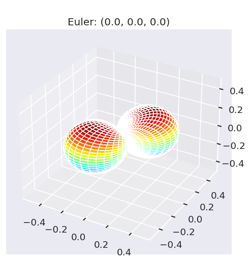
harmonics: {'dtype': 'Complex harmonics', 'kind': 'complex', 'normType':...[3]:
# Plot pol state - NOTE CURRENTLY NEED SQUEEZE HERE?
# ALSO fails for singleton case?
Itp, fig = ep.sphFromBLMPlot(linearPol.squeeze(drop=True), plotFlag = True,
backend='pl') #, facetDims=['t'])
Using complex betas (from BLMX array).
*** WARNING: plot dataset has min value < 0, min = (-0.4886025119029199+0j). This may be unphysical and/or result in plotting issues.
Sph plots:
Plotting with facetDims=None, pType=a with backend=pl.
*** Plotting for [1,1,0]
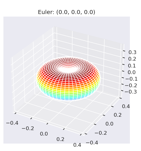
Circular polarization (\(p=\pm1\))
[4]:
# LCP = setBLMs([1,-1,1]) # Note different index
LCP = setBLMs(np.array([[1,0,0],[1,-1,1],[1,1,0]]))
Itp, fig = ep.sphFromBLMPlot(LCP.squeeze(drop=True), plotFlag = True, # pType='i',
backend='pl') #, facetDims=['t'])
Using complex betas (from BLMX array).
*** WARNING: plot dataset has min value < 0, min = (-0.34460715010224785-0.022124513098986137j). This may be unphysical and/or result in plotting issues.
Sph plots:
Plotting with facetDims=None, pType=a with backend=pl.
*** Plotting for [1,1,0]
Arb polarization
Note setting arb cases manually may not produce a realistic E-field, but is useful for testing.
[5]:
# Arb pol
arbPol = setBLMs(np.array([[1,0,0.3],[1,-1,0.4],[1,1,0.2]]))
Itp, fig = ep.sphFromBLMPlot(arbPol.squeeze(drop=True), plotFlag = True, # pType='i',
backend='pl') #, facetDims=['t'])
Using complex betas (from BLMX array).
*** WARNING: plot dataset has min value < 0, min = (-0.16198395539460675-0.00576264063312466j). This may be unphysical and/or result in plotting issues.
Sph plots:
Plotting with facetDims=None, pType=a with backend=pl.
*** Plotting for [1,1,0]
Set pol geometries (rotations)
These default to \((x,y,z)\), and are currently used either for direct frame rotation of distributions, and in MFPAD routines. Frame rotations are defined either by a set of Euler angles, or quaternions, starting from the standard orientation (\(z\)-axis vertical).
Functions:
ep.setPolGeoms() to set default or custom rotations.
ep.TKQarrayRotX() to apply the rotations (to any spherical expansion).
(See also early ePSproc frame rotation tests doc, and Quantum Metrology with Photoelectrons Vol. 1 alignment tutorial notebook.)
Formalism
For state multipoles, frame rotations are fairly straightforward (Eqn. 4.41 in Blum):
\begin{equation} \left\langle T(J',J)_{KQ}^{\dagger}\right\rangle =\sum_{q}\left\langle T(J',J)_{Kq}^{\dagger}\right\rangle D(\Omega)_{qQ}^{K*} \end{equation}
Where \(D(\Omega)_{qQ}^{K*}\) is a Wigner rotation operator, for a rotation defined by a set of Euler angles \(\Omega=\{\theta,\phi,\chi\}\). Hence the multipoles transform, as expected, as irreducible tensors, i.e. components \(q\) are mixed by rotation, but terms of different rank \(K\) are not.
For example, applying this to spherical harmonics:
\begin{equation} Y_{KQ}^{\dagger} =\sum_{q} Y_{Kq}^{\dagger} D(\Omega)_{qQ}^{K*} \end{equation}
Where \(Y_{Kq}\) is the expansion in the original frame, and \(Y_{KQ}\) in the rotated frame.
Example
[6]:
# Set default frame defns
RXdefault = ep.setPolGeoms()
RXdefault
[6]:
<xarray.DataArray (Euler: 3)>
array([quaternion(1, -0, 0, 0),
quaternion(0.707106781186548, -0, 0.707106781186547, 0),
quaternion(0.5, -0.5, 0.5, 0.5)], dtype=quaternion)
Coordinates:
* Euler (Euler) MultiIndex
- P (Euler) float64 0.0 0.0 1.571
- T (Euler) float64 0.0 1.571 1.571
- C (Euler) float64 0.0 0.0 0.0
Labels (Euler) <U32 'z' 'x' 'y'
Attributes:
dataType: Euler
mapping: canonical[7]:
# Rotations (z,x,y) case
# This transforms ep > ep' in the rotated frame
linearPolRot, _, _ = ep.TKQarrayRotX(linearPol, RXdefault)
linearPolRot
[7]:
<xarray.DataArray (t: 1, Euler: 3, BLM: 3)>
array([[[ 0.00000000e+00+0.j , 1.00000000e+00+0.j ,
0.00000000e+00+0.j ],
[ 7.07106781e-01+0.j , 2.22044605e-16+0.j ,
-7.07106781e-01+0.j ],
[ 2.00307049e-16+0.70710678j, 2.22044605e-16+0.j ,
-2.00307049e-16+0.70710678j]]])
Coordinates:
* t (t) int64 0
* Euler (Euler) MultiIndex
- P (Euler) float64 0.0 0.0 1.571
- T (Euler) float64 0.0 1.571 1.571
- C (Euler) float64 0.0 0.0 0.0
Labels (Euler) <U32 'z' 'x' 'y'
* BLM (BLM) MultiIndex
- l (BLM) int64 1 1 1
- m (BLM) int64 -1 0 1
Attributes:
dataType: BLM
long_name: Beta parameters
units: arb
harmonics: {'dtype': 'Complex harmonics', 'kind': 'complex', 'normType':...[8]:
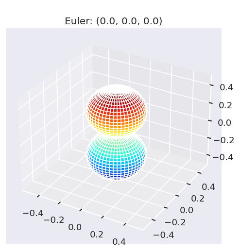
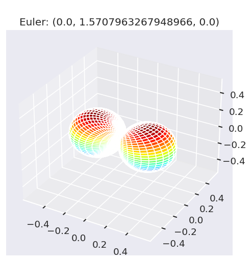
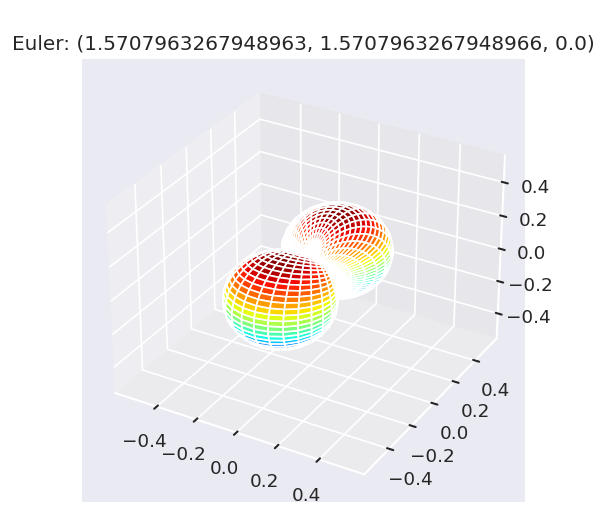
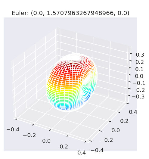
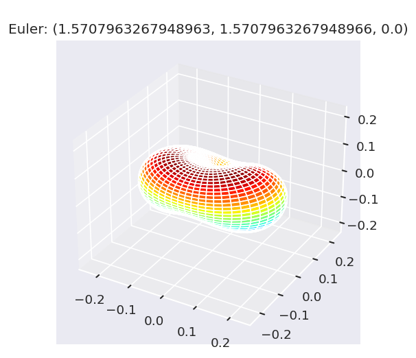
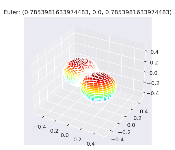
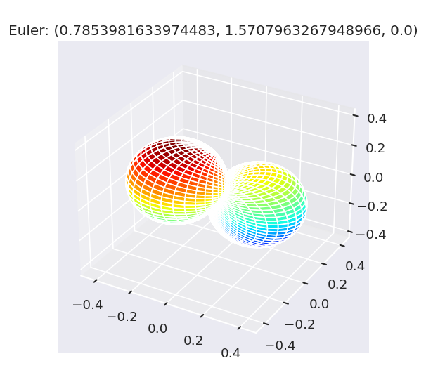
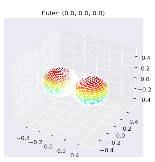
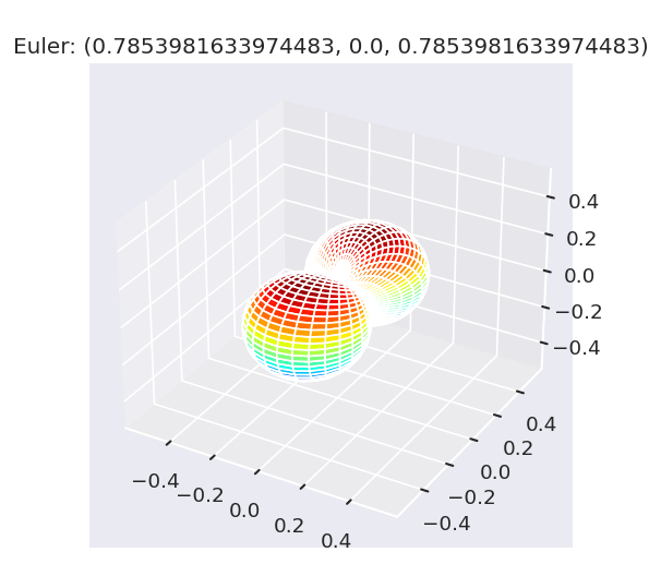
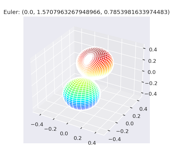
# Plot frame rotations.
# NOTE: facetDim not working for pl backend, nor for 'Labels'
# See base class .padPlot routine for better handling?
Itp, fig = ep.sphFromBLMPlot(linearPolRot.squeeze(drop=True), plotFlag = True,
backend='mpl', facetDim='Euler')
Using complex betas (from BLMX array).
*** WARNING: plot dataset has min value < 0, min = (-0.4886025119029199+0j). This may be unphysical and/or result in plotting issues.
Sph plots:
Plotting with facetDims=Euler, pType=a with backend=mpl.
Data dims: ('Euler', 'Phi', 'Theta'), subplots on Euler
Frame rotations with arb pol
These work the same way, with the caveat that LCP and RCP \(z\)-axes are usually defined as propagation direction, hence the rotated frame is usually the canonical one.
[9]:
# Rotations (z,x,y) case
LCPRot, _, _ = ep.TKQarrayRotX(LCP, RXdefault)
LCPRot
[9]:
<xarray.DataArray (t: 1, Euler: 3, BLM: 3)>
array([[[ 1.00000000e+00+0.j , 0.00000000e+00+0.j ,
0.00000000e+00+0.j ],
[ 5.00000000e-01+0.j , -7.07106781e-01+0.j ,
5.00000000e-01+0.j ],
[ 1.41638472e-16+0.5j, -7.07106781e-01+0.j ,
1.41638472e-16-0.5j]]])
Coordinates:
* t (t) int64 0
* Euler (Euler) MultiIndex
- P (Euler) float64 0.0 0.0 1.571
- T (Euler) float64 0.0 1.571 1.571
- C (Euler) float64 0.0 0.0 0.0
Labels (Euler) <U32 'z' 'x' 'y'
* BLM (BLM) MultiIndex
- l (BLM) int64 1 1 1
- m (BLM) int64 -1 0 1
Attributes:
dataType: BLM
long_name: Beta parameters
units: arb
harmonics: {'dtype': 'Complex harmonics', 'kind': 'complex', 'normType':...[10]:
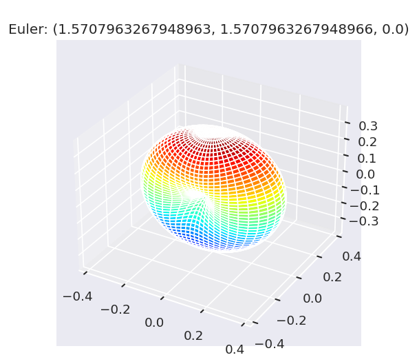
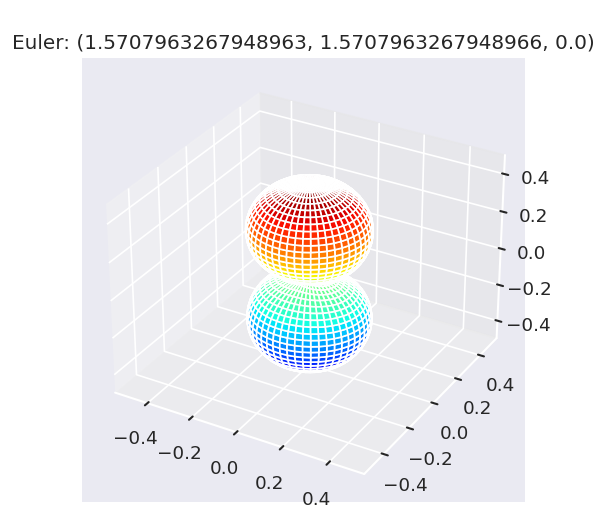
# Plot frame rotations.
# NOTE: facetDim not working for pl backend, nor for 'Labels'
# See base class .padPlot routine for better handling?
Itp, fig = ep.sphFromBLMPlot(LCPRot.squeeze(drop=True), plotFlag = True,
backend='mpl', facetDim='Euler')
Using complex betas (from BLMX array).
*** WARNING: plot dataset has min value < 0, min = (-0.34549414947133544+0j). This may be unphysical and/or result in plotting issues.
Sph plots:
Plotting with facetDims=Euler, pType=a with backend=mpl.
Data dims: ('Euler', 'Phi', 'Theta'), subplots on Euler
[11]:
# Rotations (z,x,y) case
arbPolRot, _, _ = ep.TKQarrayRotX(arbPol, RXdefault)
arbPolRot
[11]:
<xarray.DataArray (t: 1, Euler: 3, BLM: 3)>
array([[[ 4.00000000e-01+0.j , 3.00000000e-01+0.j ,
2.00000000e-01+0.j ],
[ 5.12132034e-01+0.j , -1.41421356e-01+0.j ,
8.78679656e-02+0.j ],
[ 1.45075198e-16+0.51213203j, -1.41421356e-01+0.j ,
2.48909689e-17-0.08786797j]]])
Coordinates:
* t (t) int64 0
* Euler (Euler) MultiIndex
- P (Euler) float64 0.0 0.0 1.571
- T (Euler) float64 0.0 1.571 1.571
- C (Euler) float64 0.0 0.0 0.0
Labels (Euler) <U32 'z' 'x' 'y'
* BLM (BLM) MultiIndex
- l (BLM) int64 1 1 1
- m (BLM) int64 -1 0 1
Attributes:
dataType: BLM
long_name: Beta parameters
units: arb
harmonics: {'dtype': 'Complex harmonics', 'kind': 'complex', 'normType':...[12]:
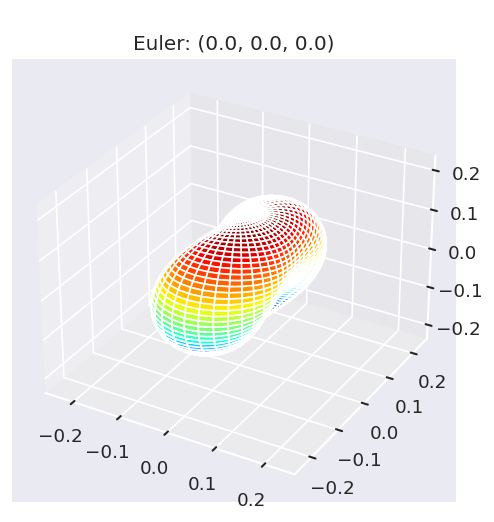
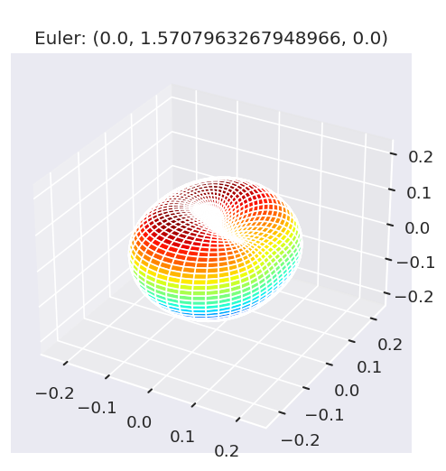
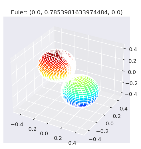
# Plot frame rotations.
# NOTE: facetDim not working for pl backend, nor for 'Labels'
# See base class .padPlot routine for better handling?
Itp, fig = ep.sphFromBLMPlot(arbPolRot.squeeze(drop=True), plotFlag = True,
backend='mpl', facetDim='Euler')
Using complex betas (from BLMX array).
*** WARNING: plot dataset has min value < 0, min = (-0.16198395539460675-0.00576264063312466j). This may be unphysical and/or result in plotting issues.
Sph plots:
Plotting with facetDims=Euler, pType=a with backend=mpl.
Data dims: ('Euler', 'Phi', 'Theta'), subplots on Euler
Pol with the Epol class
In this case, use the Epol class to define polarization states. This uses \((E_x,E_y)\) or \((E_l,E_r)\) bases for field creation, and the py_pol library for additional functionality. This provides a way to generate various arb pol fields, with the caveat that care must be taken to correctly define the reference frame.
See the main Epol class demo for details.
Linear pol with Epol class
[13]:
from epsproc.efield.epol import EfieldPol
# Define as (Ex,Ey)
Exy = EfieldPol(Exy=[1,0])
Set field from Exy.
[[1. 0.]]
[14]:
# Spherical components are set from the Ex,Ey components.
Exy.Elr
[14]:
array([[0.70710678+0.j, 0.70710678+0.j]])
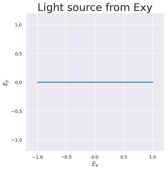
[15]:
# With py_pol, the (Ex,Ey) field can be plotted
Exy.plot()
[16]:
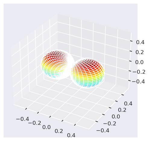
# The pol state can be expressed in Ylm basis with self.plotSph()
# This provides a quick way to check orientation relative to
# the canonical definitions above.
Exy.plotSph()
Using complex betas (from BLMX array).
*** WARNING: plot dataset has min value < 0, min = (-0.4873481053653398+0j). This may be unphysical and/or result in plotting issues.
Sph plots:
Plotting with facetDims=None, pType=a with backend=mpl.
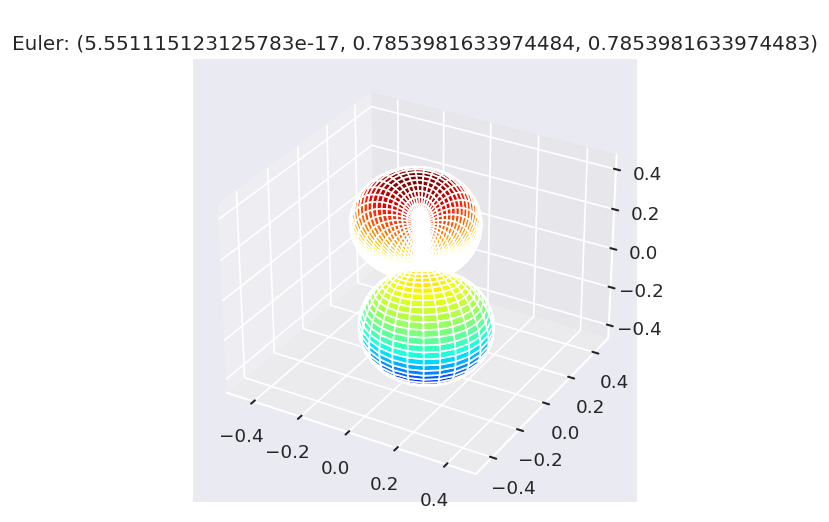
[17]:
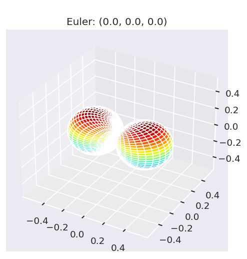
# Frame rotations are wrapped by self.setOrientation().
# For the default case this maps Ex > Ez to match the canonical frame definition.
Exy.setOrientation()
Set pol state data to self.YLM and self.YLMrot, and orientations to self.RX (mapping=exy).
[18]:
# Set 'dataType='rot'' to plot the rotated frames.
Exy.plotSph(dataType='rot')
Using complex betas (from BLMX array).
*** WARNING: plot dataset has min value < 0, min = (-0.4886025119029198+0j). This may be unphysical and/or result in plotting issues.
Sph plots:
Plotting with facetDims=Euler, pType=a with backend=mpl.
Data dims: ('Euler', 'Phi', 'Theta'), subplots on Euler

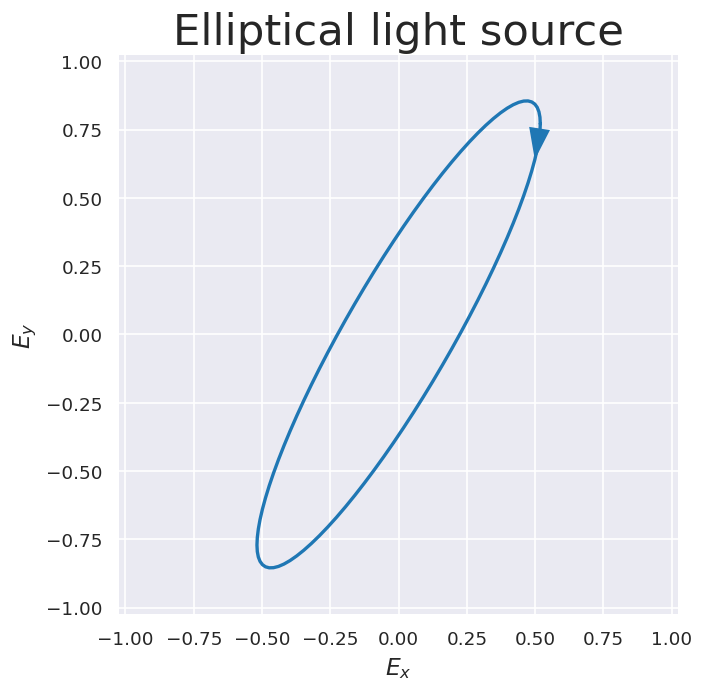
Elliptical pol with Epol class
For the elliptical case, it can be specified by parameters [amplitude,azimuth (0,pi), ellipticity (-pi/4,pi/4)]. (See the main Epol class docs for more details.)
[19]:
import numpy as np
# Define circ pol fields (max and min ellipticity)
Eell_RCP = EfieldPol(ell=[1,0,np.pi/4])
Eell_LCP = EfieldPol(ell=[1,0,-np.pi/4])
# Define arb ellipticity
Eell_mixed = EfieldPol(ell=[1,0,0.25*np.pi/4])
Eell_rotated = EfieldPol(ell=[1,np.pi/3,0.25*np.pi/4])
Set field from ell.
[[1. 0. 0.78539816]]
Set field from ell.
[[ 1. 0. -0.78539816]]
Set field from ell.
[[1. 0. 0.19634954]]
Set field from ell.
[[1. 1.04719755 0.19634954]]
[20]:
# Check field
Eell_rotated.plot()
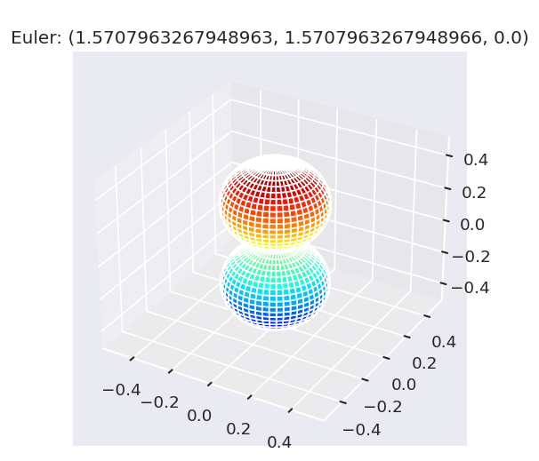
Eell_rotated.plotSph()
Using complex betas (from BLMX array).
*** WARNING: plot dataset has min value < 0, min = (-0.45384144299916224-0.14775656726827413j). This may be unphysical and/or result in plotting issues.
Sph plots:
Plotting with facetDims=None, pType=a with backend=mpl.
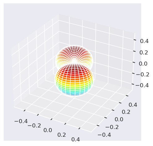
[21]:
# Set/map frame to default geoms
# Frame rotations are wrapped by self.setOrientation().
# For the default case this maps Ex > Ez to match the canonical frame definition.
Eell_rotated.setOrientation()
# Set 'dataType='rot'' to plot the rotated frames.
Eell_rotated.plotSph(dataType='rot')
Set pol state data to self.YLM and self.YLMrot, and orientations to self.RX (mapping=exy).
Using complex betas (from BLMX array).
*** WARNING: plot dataset has min value < 0, min = (-0.4538564795163548+0.15098416308662488j). This may be unphysical and/or result in plotting issues.
Sph plots:
Plotting with facetDims=Euler, pType=a with backend=mpl.
Data dims: ('Euler', 'Phi', 'Theta'), subplots on Euler


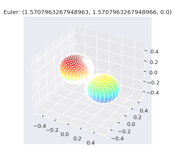
Note in this case that the default mapping maintains the diagonal polarization state in the \((x,z)\) plane in the final transformation.
Arb frame rotations with Epol class
In somes cases, the default rotations may not be what we want, so we can set manually instead…
[22]:
# Test alternative z mappings - custom case
pRot = [0, np.pi/2, np.pi/4]
tRot = [0, 0, np.pi/2]
cRot = [0, 0, 0]
labels = ['x', 'y', 'z']
eulerAngsEpol = np.array([pRot, tRot, cRot]).T
RXEpol=ep.setPolGeoms(eulerAngs = eulerAngsEpol, labels = labels)
Eell_rotated.setOrientation(RX=RXEpol)
# Set 'dataType='rot'' to plot the rotated frames.
Eell_rotated.plotSph(dataType='rot')
Set pol state data to self.YLM and self.YLMrot, and orientations to self.RX (mapping=exy).
Using complex betas (from BLMX array).
*** WARNING: plot dataset has min value < 0, min = (-0.4538564795163548+0.15098416308662488j). This may be unphysical and/or result in plotting issues.
Sph plots:
Plotting with facetDims=Euler, pType=a with backend=mpl.
Data dims: ('Euler', 'Phi', 'Theta'), subplots on Euler
[23]:
# Set mappings using those available in ep.setPolGeoms()
# Set mapping including "diagonal" pol geometries
Eell_mixed.setOrientation(mapping='exyDiag')
Eell_mixed.plotSph(dataType='rot')
Set pol state data to self.YLM and self.YLMrot, and orientations to self.RX (mapping=exyDiag).
Using complex betas (from BLMX array).
*** WARNING: plot dataset has min value < 0, min = (-0.479214151642428+0j). This may be unphysical and/or result in plotting issues.
Sph plots:
Plotting with facetDims=Euler, pType=a with backend=mpl.
Data dims: ('Euler', 'Phi', 'Theta'), subplots on Euler
Molecular frame example (\(N_2\))
Quick demo as per the main class intro docs.
Import matrix elements
[24]:
# Import
import epsproc as ep
from pathlib import Path
# Set data path
# Note this is set here from ep.__path__, but may not be correct in all cases - depends on where the Github repo is.
epDemoDataPath = Path(ep.__path__[0]).parent/'data'
dataPath = epDemoDataPath/'photoionization'/'n2_multiorb'
[25]:
# Class dev code
from epsproc.classes.multiJob import ePSmultiJob
from epsproc.classes.base import ePSbase
# Instantiate class object.
# Minimally this needs just the dataPath, if verbose = 1 is set then some useful output will also be printed.
data = ePSbase(dataPath, verbose = 1)
# ScanFiles() - this will look for data files on the path provided, and read from them.
data.scanFiles()
*** Job orb6 details
Key: orb6
Dir /home/jovyan/code-share/github-share/ePSproc/data/photoionization/n2_multiorb, 1 file(s).
{ 'batch': 'ePS n2, batch n2_1pu_0.1-50.1eV, orbital A2',
'event': ' N2 A-state (1piu-1)',
'orbE': -17.09691397835426,
'orbLabel': '1piu-1'}
*** Job orb5 details
Key: orb5
Dir /home/jovyan/code-share/github-share/ePSproc/data/photoionization/n2_multiorb, 1 file(s).
{ 'batch': 'ePS n2, batch n2_3sg_0.1-50.1eV, orbital A2',
'event': ' N2 X-state (3sg-1)',
'orbE': -17.34181645456815,
'orbLabel': '3sg-1'}
[26]:
# Plot molecule
data.molSummary()
*** Molecular structure
*** Molecular orbital list (from ePS output file)
EH = Energy (Hartrees), E = Energy (eV), NOrbGrp, OrbGrp, GrpDegen = degeneracies and corresponding orbital numbering by group in ePS, NormInt = single centre expansion convergence (should be ~1.0).
| props | Sym | EH | Occ | E | NOrbGrp | OrbGrp | GrpDegen | NormInt |
|---|---|---|---|---|---|---|---|---|
| orb | ||||||||
| 1 | SG | -15.6719 | 2.0 | -426.454124 | 1.0 | 1.0 | 1.0 | 0.999532 |
| 2 | SU | -15.6676 | 2.0 | -426.337115 | 1.0 | 2.0 | 1.0 | 0.999458 |
| 3 | SG | -1.4948 | 2.0 | -40.675580 | 1.0 | 3.0 | 1.0 | 0.999979 |
| 4 | SU | -0.7687 | 2.0 | -20.917393 | 1.0 | 4.0 | 1.0 | 0.999979 |
| 5 | SG | -0.6373 | 2.0 | -17.341816 | 1.0 | 5.0 | 1.0 | 1.000000 |
| 6 | PU | -0.6283 | 2.0 | -17.096914 | 1.0 | 6.0 | 2.0 | 1.000000 |
| 7 | PU | -0.6283 | 2.0 | -17.096914 | 2.0 | 6.0 | 2.0 | 1.000000 |
Compute MFPADs
Note that the MF routine will compute for all passed polarization geometries by default, but additional control is available by setting and subselecting from the Epol class object prior to passing it to the MF computational function.
[27]:
# Use Epol class object as Einput, just needs self.epDict to be passed.
# Einput = Eell_rotated
# Einput = Eell_mixed
Einput = Exy
# # Set params for MFBLM calculation
# Einput.setep()
# Einput.setOrientation() # To ensure frame settings for Epol, run self.setOrientation.
# # Otherwise MFBLM computation will use defaults.
# # Run standard calculation with inputs from Epol
# data.MFBLM(**Einput.epDict)
# Update March 2024 - can now also just pass E-field class object directly, although may still want the above for additional control
data.MFBLM(EfieldPol = Einput)
Calculating MF-BLMs for job key: orb6
Set E-field parameters to `self.epDict` and `self.epXR`, using basis=ep (rotSel=None).
Calculating MF-BLMs for job key: orb5
[28]:
# data.BLMplot(dataType='MFBLM', thres = 1e-2, backend='hv', Erange=[0,15], ylim=(-1.5, 2.5), width=800)
data.padPlot(keys = 'orb5', Erange = [5, 10, 4], dataType='MFBLM', backend='pl', returnFlag=True) #, facetDims=['Eke','Labels']) #['Eke','Labels'])
Using default sph betas.
Summing over dims: set()
Plotting from self.data[orb5][MFBLM], facetDims=['Eke', 'Labels'], pType=a with backend=pl.
*** WARNING: plot dataset has min value < 0, min = (-2.9550010003161643e-06-1.7929644151886635e-18j). This may be unphysical and/or result in plotting issues.
*** WARNING: plot dataset has min value < 0, min = (-1.4325621678853181e-05+6.599682751978262e-18j). This may be unphysical and/or result in plotting issues.
Set plot to self.data['orb5']['plots']['MFBLM']['polar']
Aligned frame (AF) PAD example
For the AF case, the same methodology applies, except that the calculations currently only support a single E-field polarization geometry, which needs to be set prior to the calculations.
This is included as of 22/05/24. The default cases sets the z-axis as the main polarization axis (which matches the ADM expansion), and can be overridden by passing additional parameters. This is illustrated below.
Set alignment (ADMs)
Here load sample ADMs for N2 for testing.
See the class docs for more details.
[29]:
from epsproc.classes.alignment import ADM
# Set dir and file type
epDemoDataPath = Path(ep.__path__[0]).parent/'data' # Note this may also need `.expanduser()` to be set for full path.
dataPath = epDemoDataPath/'alignment'
ADMtype = '.mat'
# Create object
ADMin = ADM(fileBase=dataPath, ext = ADMtype)
# Read file
ADMin.loadData()
# Plot ADMs
ADMin.plot()
Scanning /home/jovyan/code-share/github-share/ePSproc/data/alignment for ePS jobs.
Found ePS output files in subdirs: [PosixPath('/home/jovyan/code-share/github-share/ePSproc/data/alignment/C2H4_ADMs_8TW_120fs_VM')]
Found ePS output files in root dir /home/jovyan/code-share/github-share/ePSproc/data/alignment.
*** Scanning dir
/home/jovyan/code-share/github-share/ePSproc/data/alignment
Found 1 .mat file(s)
Files from self.fileDict read OK, outputs: self.dataDict and self.data.
[30]:
# Subselection and downsample for calculations
ADMin.subsetADMs(trange=[6,10],tStep = 5, plotSubset=True)
Setting subset data from `self.data['alignment']['ADM']`
*** Warning: setting ADMs with ndim = 3 may cause issues. Trying squeeze to fix...
Squeezed OK
Selecting 41 points
Set subset data to `self.data['ADM']['ADM']`
Compute AFPADs
Note that the AF routine will compute for only a single polarization geometry (although multiple polarization states are supported), and will use the z-pol case by default, but additional control is available by setting and subselecting from the Epol class object prior to passing it to the MF computational function.
[31]:
# Use Epol class object as Einput, just needs self.epDict to be passed.
# Einput = Eell_rotated
# Einput = Eell_mixed
Einput = Exy
# With pol...
# data.AFBLM(AKQS = ADMin.data['ADM']['ADM'], EfieldPol = Einput, thres=1e-4)
# selDims = {'Type':'L'}, thres=thres)
data.AFBLM(AKQS = ADMin, EfieldPol = Einput, thres=1e-4)
Calculating AF-BLMs for job key: orb6
Set E-field parameters to `self.epDict` and `self.epXR`, using basis=rot (rotSel=z).
Using ADMs from AKQS.data['ADM']['ADM']
Calculating AF-BLMs for job key: orb5
Set E-field parameters to `self.epDict` and `self.epXR`, using basis=rot (rotSel=z).
Using ADMs from AKQS.data['ADM']['ADM']
[32]:
# data.BLMplot(dataType='AFBLM', thres = 1e-2) # Passing a threshold value here will remove any spurious BLM parameters.
# Set data - use existing plot routine but skip line outs (quite slow, replotted at end of notebook)
# data.BLMplot(backend='hv', xDim = 't', renderPlot=False, pl)
data.BLMplot(backend='hv', xDim = 't', hvType='heatmap') #, addHist = True, addADMs = False, XS=False) #, clim=(-1,2))
BLMplot set data and plots to self.plots['BLMplot']
WARNING:param.HeatMapPlot03211: Due to internal constraints, when aspect and width/height is set, the bokeh backend uses those values as frame_width/frame_height instead. This ensures the aspect is respected, but means that the plot might be slightly larger than anticipated. Set the frame_width/frame_height explicitly to suppress this warning.
[32]:
True
Using a non-default frame for AF calculations
Optional - either pass subselection from default cases at AF calculation, or set prior to calculation.
[33]:
# Using a different default case
data.AFBLM(AKQS = ADMin, EfieldPol = Einput, thres=1e-4, EfieldRotSel = 'x')
data.BLMplot(backend='hv', xDim = 't', hvType='heatmap', addADMs = True)
Calculating AF-BLMs for job key: orb6
Set E-field parameters to `self.epDict` and `self.epXR`, using basis=rot (rotSel=x).
Using ADMs from AKQS.data['ADM']['ADM']
Calculating AF-BLMs for job key: orb5
Set E-field parameters to `self.epDict` and `self.epXR`, using basis=rot (rotSel=x).
Using ADMs from AKQS.data['ADM']['ADM']
BLMplot set data and plots to self.plots['BLMplot']
WARNING:param.HeatMapPlot05892: Due to internal constraints, when aspect and width/height is set, the bokeh backend uses those values as frame_width/frame_height instead. This ensures the aspect is respected, but means that the plot might be slightly larger than anticipated. Set the frame_width/frame_height explicitly to suppress this warning.
[33]:
True
[34]:
# Using a pre-set case, here can use either a mapping or set of Euler angles as illustrated previously.
# Set params for AFBLM calculation, with diagonal cases
Einput.setOrientation(mapping='exyDiag')
# Einput.setOrientation() # To ensure frame settings for Epol, run self.setOrientation.
# # Otherwise MFBLM computation will use defaults.
data.AFBLM(AKQS = ADMin, EfieldPol = Einput, thres=1e-4, EfieldRotSel = '+45x')
data.BLMplot(backend='hv', xDim = 't', hvType='heatmap', XS=True, clim = (-1,2)) # Note clim passing here, and XS=True to show XS
# Note - for some pol geometries small values might cause normalisation issues.
# Setting clim - as above - will highlight unphysical outputs.
# Filtering on XS may also help, e.g. pass `filterXS=1e-2`
Set pol state data to self.YLM and self.YLMrot, and orientations to self.RX (mapping=exyDiag).
Set orientations to self.epDict['RX'].
Calculating AF-BLMs for job key: orb6
Set E-field parameters to `self.epDict` and `self.epXR`, using basis=rot (rotSel=+45x).
Using ADMs from AKQS.data['ADM']['ADM']
Calculating AF-BLMs for job key: orb5
Set E-field parameters to `self.epDict` and `self.epXR`, using basis=rot (rotSel=+45x).
Using ADMs from AKQS.data['ADM']['ADM']
BLMplot set data and plots to self.plots['BLMplot']
WARNING:param.HeatMapPlot09164: Due to internal constraints, when aspect and width/height is set, the bokeh backend uses those values as frame_width/frame_height instead. This ensures the aspect is respected, but means that the plot might be slightly larger than anticipated. Set the frame_width/frame_height explicitly to suppress this warning.
[34]:
True
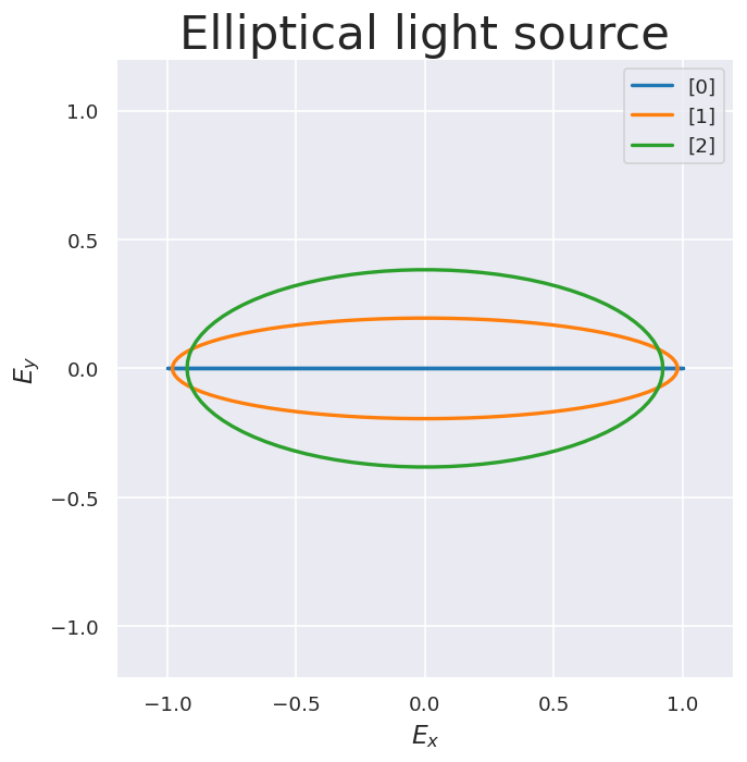
Using multiple polarization states
In general, this should be handled transparently… in the default case the polarization states will be labelled by the EfieldPol labels.
[35]:
# Mulitple ellipticities and rotations
# For fields, set with format = [amplitude,azimuth (0,pi), ellipticity (-pi/4,pi/4)]
states = 3
# angles = np.linspace(0, np.pi, states) # For range of angles
angles = np.zeros(states) # no rotation
maxEll = 0.5 # Set max ellipticity to use (0 - 1)
ellipticities = np.linspace(0,maxEll*np.pi/4, states) # Set for 0 - max ellipticity
ell = np.c_[np.ones(states),angles,ellipticities]
labels = (ellipticities/(np.pi/4) * 100).round(2) # Set labels at %age ellipticity
# Set fields
Eell_multi = EfieldPol(ell=ell, labels = labels)
# Plot fields
Eell_multi.plot(figsize=(6,6), draw_arrow=False)
# plt.legend(labels, loc='upper right')
Set field from ell.
[[1. 0. 0. ]
[1. 0. 0.19634954]
[1. 0. 0.39269908]]
[36]:
# Use Epol class object as Einput, just needs self.epDict to be passed.
# Einput = Eell_rotated
# Einput = Eell_mixed
# Einput = Exy
Einput = Eell_multi
# With pol...
data.AFBLM(AKQS = ADMin.data['ADM']['ADM'], EfieldPol = Einput, thres=1e-4)
Calculating AF-BLMs for job key: orb6
Set pol state data to self.YLM and self.YLMrot, and orientations to self.RX (mapping=exy).
Skipping self.epXR configuration, issue with dims.
Set E-field parameters to `self.epDict` and `self.epXR`, using basis=rot (rotSel=z).
Set geomCalc.EPR() results to `self.EPRX`.
Calculating AF-BLMs for job key: orb5
Skipping self.epXR configuration, issue with dims.
Set E-field parameters to `self.epDict` and `self.epXR`, using basis=rot (rotSel=z).
Set geomCalc.EPR() results to `self.EPRX`.
Versions
[37]:
import scooby
scooby.Report(additional=['epsproc', 'holoviews', 'hvplot', 'xarray', 'matplotlib', 'bokeh', 'plotly'])
[37]:
| Mon May 27 11:54:43 2024 EDT | |||||||
| OS | Linux | CPU(s) | 64 | Machine | x86_64 | Architecture | 64bit |
| RAM | 62.8 GiB | Environment | Jupyter | File system | btrfs | ||
| Python 3.10.11 | packaged by conda-forge | (main, May 10 2023, 18:58:44) [GCC 11.3.0] | |||||||
| epsproc | 1.3.2-dev | holoviews | 1.16.2 | hvplot | 0.8.4 | xarray | 2022.3.0 |
| matplotlib | 3.5.3 | bokeh | 3.1.1 | plotly | 5.15.0 | numpy | 1.23.5 |
| scipy | 1.10.1 | IPython | 8.13.2 | scooby | 0.7.2 | ||
[38]:
# Check current Git commit for local ePSproc version
from pathlib import Path
!git -C {Path(ep.__file__).parent} branch
!git -C {Path(ep.__file__).parent} log --format="%H" -n 1
* 3d-AFPAD-dev
dev
master
ccea2599f0980082cee8d76736f909c25ab87f3d
[39]:
# Check current remote commits
!git ls-remote --heads https://github.com/phockett/ePSproc
1e28825260d558625d1dae6f7aa637513246ebbc refs/heads/3d-AFPAD-dev
18901ac6056324d6a2674396939fdcc373d35395 refs/heads/dependabot/pip/notes/envs/envs-versioned/idna-3.7
9d9eb4e1a20d4ff77d07af2ac782ba18c26e5dcc refs/heads/dependabot/pip/notes/envs/envs-versioned/jinja2-3.1.4
226759a58ebe96bf1a6df60ccd5efb0c449af3a7 refs/heads/dependabot/pip/notes/envs/envs-versioned/pillow-10.3.0
de0e271701949602ce7f170a9665e37b27d2401c refs/heads/dependabot/pip/notes/envs/envs-versioned/requests-2.32.0
4ff0ed84a1df2a3de4258ba7e49db1e47e6ac596 refs/heads/dependabot/pip/notes/envs/envs-versioned/scipy-1.11.1
b50b0b946a1a7cb5b22c95d1e4cee120b22e6874 refs/heads/dependabot/pip/notes/envs/envs-versioned/tqdm-4.66.3
fd9c621f0c91e05ffcb097f59e9d8d8b43c5fc23 refs/heads/dependabot/pip/scipy-1.11.1
7e4270370d66df44c334675ac487c87d702408da refs/heads/dev
1c0b8fd409648f07c85f4f20628b5ea7627e0c4e refs/heads/master
69cd89ce5bc0ad6d465a4bd8df6fba15d3fd1aee refs/heads/numba-tests
ea30878c842f09d525fbf39fa269fa2302a13b57 refs/heads/revert-9-master
baf0be0c962e8ab3c3df57c8f70f0e939f99cbd7 refs/heads/testDev
[ ]: