Density Matrices notes + demo (ePSproc + PEMtk dev.)
30/08/21, 24/07/24
In this notebook density matrices are considered & numerical routines demonstrated.
24/07/24: Updated notes and added density matrix from spherical tensor example.
Density Matrices
The general density operator, for a mixture of indepent states \(|\psi_{n} \rangle\), can be defined as (Eqn. 2.8, Blum [1]):
\begin{equation} \hat{\rho}=\sum_{n}W_{n}|\psi_{n}\rangle\langle\psi_{n}| \end{equation}
Where \(W_{n}\) defines the (statistical) weighting of each state \(\psi_{n}\) in the mixture.
For a given basis set, \(|\phi_{m}\rangle\), the states can be expanded and the matrix elements of \(\boldsymbol{\rho}\) defined (Eqns. 2.9 - 2.11, Blum [1]): \begin{equation} | \psi_{n} \rangle = \sum_{m'} a_{m'}^{(n)}| \phi_{m'}\rangle \end{equation}
\begin{equation} \hat{\rho}=\sum_{n}\sum_{mm'}W_{n}a_{m'}^{(n)}a_{m}^{(n)*}|\phi_{m'}\rangle\langle\phi_{m}| \end{equation}
And the matrix elements - the density matrix - given explicitly as:
\begin{equation} \boldsymbol{\rho}_{i,j}=\langle\phi_{i}|\hat{\rho}|\phi_{j}\rangle=\sum_{n}W_{n}a_{i}^{(n)}a_{j}^{(n)*} \end{equation}
For all pairs of basis states \((i,j)\). This defines the density matrix in the \(\{|\phi_n\rangle\}\) representation (basis space).
The expectation value of an operator \(\hat{Q}\) can then be found as (Eqn. 2.18, Blum [1]):
:nbsphinx-math:`begin{eqnarray} langle hat{Q}rangle & = & sum_{n}sum_{mm’}W_{n}a_{m’}^{(n)}a_{m}^{(n)*}langlephi_{m}|hat{Q}|phi_{m’}rangle\
& = & sum_{mm’}langlephi_{m’}|hat{rho}|phi_{m}ranglelanglephi_{m}|hat{Q}|phi_{m’}rangle\ & = & mathrm{tr}(rho Q)
end{eqnarray}`
For basic examples, in terms of \(|J,M\rangle\) states and alignment, see the Quantum Metrology with Photoelectrons notes.
Here, we’ll look at applying the formalism to photoionization, using ePSproc for the numerics…
[1] Blum, K. (2012). Density Matrix Theory and Applications (3rd Editio, Vol. 64). Berlin, Heidelberg: Springer Berlin Heidelberg. https://doi.org/10.1007/978-3-642-20561-3
Setup
[1]:
import sys
import os
from pathlib import Path
import numpy as np
# import epsproc as ep
import xarray as xr

import matplotlib.pyplot as plt

from datetime import datetime as dt
timeString = dt.now()

import epsproc as ep

# Multijob class dev code
from epsproc.classes.multiJob import ePSmultiJob
OMP: Info #276: omp_set_nested routine deprecated, please use omp_set_max_active_levels instead.
* sparse not found, sparse matrix forms not available.
* natsort not found, some sorting functions not available.
* Setting plotter defaults with epsproc.basicPlotters.setPlotters(). Run directly to modify, or change options in local env.
* Set Holoviews with bokeh.
* pyevtk not found, VTK export not available.
[2]:
epDemoDataPath = Path(ep.__path__[0]).parent/'data'/'photoionization'/'n2_multiorb'
Load test data
[3]:
# Class dev code
from epsproc.classes.multiJob import ePSmultiJob
from epsproc.classes.base import ePSbase

# Instantiate class object.
# Minimally this needs just the dataPath, if verbose = 1 is set then some useful output will also be printed.
data = ePSbase(epDemoDataPath, verbose = 1)

# ScanFiles() - this will look for data files on the path provided, and read from them.
data.scanFiles()
*** Job orb6 details
Key: orb6
Dir /home/jovyan/code-share/github-share/ePSproc/data/photoionization/n2_multiorb, 1 file(s).
{   'batch': 'ePS n2, batch n2_1pu_0.1-50.1eV, orbital A2',
    'event': ' N2 A-state (1piu-1)',
    'orbE': -17.09691397835426,
    'orbLabel': '1piu-1'}

*** Job orb5 details
Key: orb5
Dir /home/jovyan/code-share/github-share/ePSproc/data/photoionization/n2_multiorb, 1 file(s).
{   'batch': 'ePS n2, batch n2_3sg_0.1-50.1eV, orbital A2',
    'event': ' N2 X-state (3sg-1)',
    'orbE': -17.34181645456815,
    'orbLabel': '3sg-1'}
Density matrix functions - demo with photoionization matrix elements
As of ePSproc v1.3.1-dev commit f5e4019, density matrix routines are implemented in :py:func:epsproc.calc.density (functional forms only).
Note this currently requires Holoviews for plotting.
[4]:
# Import routines
from epsproc.calc import density


Set data
The routines are not currently wrapped by the main data class, so we’ll just use a single sample dataset here.
[5]:
# Set data from master class
k = 'orb5'  # N2 orb5 (SG) dataset
matE = data.data[k]['matE']
selDims = {'Type':'L'}
thres = 1e-2
[6]:
# Check data with lmPlot()
ep.lmPlot(matE, selDims = selDims, thres = thres);
Plotting data n2_3sg_0.1-50.1eV_A2.inp.out, pType=a, thres=0.01, with Seaborn

Calculate density matrix
The numerics essentially computer the outer product from the specified dimensions, as per the previous definition:
\begin{equation} \boldsymbol{\rho}_{i,j}=\langle\phi_{i}|\hat{\rho}|\phi_{j}\rangle=\sum_{n}W_{n}a_{i}^{(n)}a_{j}^{(n)*} \end{equation}
where \(a_{i}^{(n)}a_{j}^{(n)*}\) are the values along the specified dimensions/state vector/representation. These dimensions must be in data, but will be restacked as necessary to define the effective basis space. For instance, from the ionization matrix element data shown above, setting [l,m] would select the \(|\alpha\rangle = |l,m\rangle\) basis (equivalently LM, since the dimensions are already stacked in the ionization matrix elements). Setting ['LM','mu'] would set the
\(|\alpha\rangle = |l,m,\mu\rangle\) as the basis vector and so forth, where \(|\alpha\rangle\) is used as a generic state vector denoting all required quantum numbers.
Note, however, that this selection is purely based on the numerics, which computes the outer product \(|\alpha\rangle\langle\alpha'|\) to form the density matrix, hence does not guarantee a well-formed density matrix in the strictest sense (depending on the basis set), although will always present a basis state correlation matrix of sorts.
[7]:
# Compose density matrix

# Set dimensions/state vector/representation
# These must be in original data, but will be restacked as necessary to define the effective basis space.
denDims = ['LM', 'mu']

# Calculate
daOut, *_ = density.densityCalc(matE, denDims = denDims, selDims = selDims, thres = thres)  # OK
[8]:
# The output is an Xarray, with a square density matrix in the specified dims (alpha, alpha'), where the latter is labelled '_p'.
# Other dims will be automatically stacked (unless otherwise specified).
daOut
[8]:
<xarray.DataArray 'n2_3sg_0.1-50.1eV_A2.inp.out' (Eke: 51, Sym: 2, l,m,mu: 9,
                                                  l,m,mu_p: 9)>
array([[[[        nan       +nanj,         nan       +nanj,
                  nan       +nanj, ...,         nan       +nanj,
                  nan       +nanj,         nan       +nanj],
         [        nan       +nanj,  7.49604313+0.j        ,
                  nan       +nanj, ...,         nan       +nanj,
                  nan       +nanj,         nan       +nanj],
         [        nan       +nanj,         nan       +nanj,
                  nan       +nanj, ...,         nan       +nanj,
                  nan       +nanj,         nan       +nanj],
         ...,
         [        nan       +nanj,         nan       +nanj,
                  nan       +nanj, ...,         nan       +nanj,
                  nan       +nanj,         nan       +nanj],
         [        nan       +nanj,         nan       +nanj,
                  nan       +nanj, ...,         nan       +nanj,
                  nan       +nanj,         nan       +nanj],
         [        nan       +nanj,         nan       +nanj,
                  nan       +nanj, ...,         nan       +nanj,
                  nan       +nanj,         nan       +nanj]],

...

        [[ 0.66738586+0.j        ,         nan       +nanj,
           0.66738586+0.j        , ..., -0.08467309+0.06156213j,
                  nan       +nanj, -0.08467309+0.06156213j],
         [        nan       +nanj,         nan       +nanj,
                  nan       +nanj, ...,         nan       +nanj,
                  nan       +nanj,         nan       +nanj],
         [ 0.66738586+0.j        ,         nan       +nanj,
           0.66738586+0.j        , ..., -0.08467309+0.06156213j,
                  nan       +nanj, -0.08467309+0.06156213j],
         ...,
         [-0.08467309-0.06156213j,         nan       +nanj,
          -0.08467309-0.06156213j, ...,  0.01642143+0.j        ,
                  nan       +nanj,  0.01642143+0.j        ],
         [        nan       +nanj,         nan       +nanj,
                  nan       +nanj, ...,         nan       +nanj,
                  nan       +nanj,         nan       +nanj],
         [-0.08467309-0.06156213j,         nan       +nanj,
          -0.08467309-0.06156213j, ...,  0.01642143+0.j        ,
                  nan       +nanj,  0.01642143+0.j        ]]]])
Coordinates:
    Type      <U1 'L'
  * Sym       (Sym) MultiIndex
  - Cont      (Sym) object 'SU' 'PU'
  - Targ      (Sym) object 'SG' 'SG'
  - Total     (Sym) object 'SU' 'PU'
  * Eke       (Eke) float64 0.1 1.1 2.1 3.1 4.1 5.1 ... 46.1 47.1 48.1 49.1 50.1
    Ehv       (Eke) float64 17.4 18.4 19.4 20.4 21.4 ... 64.4 65.4 66.4 67.4
    SF        (Eke) complex128 (2.1560627+3.741674j) ... (4.4127053+1.8281945j)
  * l,m,mu    (l,m,mu) MultiIndex
  - l         (l,m,mu) int64 1 1 1 3 3 3 5 5 5
  - m         (l,m,mu) int64 -1 0 1 -1 0 1 -1 0 1
  - mu        (l,m,mu) int64 1 0 -1 1 0 -1 1 0 -1
  * l,m,mu_p  (l,m,mu_p) MultiIndex
  - l_p       (l,m,mu_p) int64 1 1 1 3 3 3 5 5 5
  - m_p       (l,m,mu_p) int64 -1 0 1 -1 0 1 -1 0 1
  - mu_p      (l,m,mu_p) int64 1 0 -1 1 0 -1 1 0 -1
Attributes:
    dataType:  Density Matrix
    file:      n2_3sg_0.1-50.1eV_A2.inp.out
    fileBase:  /home/jovyan/code-share/github-share/ePSproc/data/photoionizat...
    fileList:  n2_3sg_0.1-50.1eV_A2.inp.out
    jobLabel:  3sg-1
    density:   {'denSettings': {'da': <xarray.DataArray 'n2_3sg_0.1-50.1eV_A2...
kdims: ['l,m,mu', 'l,m,mu_p']Plotting density matrices
This is handled by the matPlot() routine. This uses Holoviews to compose a full-dimensional plot, as a set of matrices in the key dimensions \([\alpha,\alpha']\), and stacked in other dimensions. The plots are interactive + widgets for control, or can be pushed to a layout with Holoviews functionality.
[9]:
# Plot full matrix
# This is interactive (with Holoviews), with the widgets allowing selection of other (stacked) dimensions.
# Plot types [real, imag, abs] are also set.
# Note this may take a while for data with a large number of dimensions.
density.matPlot(daOut)
Set plot kdims to ['l,m,mu', 'l,m,mu_p']; pass kdims = [dim1,dim2] for more control.
WARNING:param.HeatMapPlot03274: Due to internal constraints, when aspect and width/height is set, the bokeh backend uses those values as frame_width/frame_height instead. This ensures the aspect is respected, but means that the plot might be slightly larger than anticipated. Set the frame_width/frame_height explicitly to suppress this warning.
[9]:
[10]:
# For more control, the Xarray and/or Holoviews object can be manipulated prior to plotting

hvmap = density.matPlot(daOut.sum('Sym').sel(Eke=slice(5,50,20)))  # Sum & slice data prior to plot
                                                                    # Note that summation may replace NaNs with zeros.
hvmap.layout('Eke').cols(1)  # Layout results by Eke, single column layout
WARNING:param.HeatMapPlot261168: Due to internal constraints, when aspect and width/height is set, the bokeh backend uses those values as frame_width/frame_height instead. This ensures the aspect is respected, but means that the plot might be slightly larger than anticipated. Set the frame_width/frame_height explicitly to suppress this warning.
WARNING:param.HeatMapPlot261174: Due to internal constraints, when aspect and width/height is set, the bokeh backend uses those values as frame_width/frame_height instead. This ensures the aspect is respected, but means that the plot might be slightly larger than anticipated. Set the frame_width/frame_height explicitly to suppress this warning.
WARNING:param.HeatMapPlot261179: Due to internal constraints, when aspect and width/height is set, the bokeh backend uses those values as frame_width/frame_height instead. This ensures the aspect is respected, but means that the plot might be slightly larger than anticipated. Set the frame_width/frame_height explicitly to suppress this warning.
Set plot kdims to ['l,m,mu', 'l,m,mu_p']; pass kdims = [dim1,dim2] for more control.
[10]:
TODO:
Cmapping & dynamic map range control.
NaN replacement issues?
Normalisation.
Density matrices from other data types
As defined above, an approximate density/correlation matrix can be composed from any Xarray. Strictly speaking, this may not always provide a well-formed density matrix, but will always provide a correlation matrix which may be interesting/informative for a given case.
Here we’ll look at some other data-types, using the AF-BLM routine (strictly speaking, this defines a set of geometric tensors, which may have a direct relation with the corresponding density matrix - this will be explored below, here we’ll just do the numerics). For an more details of the AF-BLM routine see the theory notes and the basis set exploration page. (Note 24/07/24 update: results here are slightly different to previously, since AFBLM code now defaults to p=0/z-pol case, so R=0 terms only in default case.)
[11]:
# Calculate AFPADs with full basis set return
# The default case will compute LF-BLM parameters
BetasNormX, basis = ep.afblmXprod(matE, selDims=selDims, basisReturn='Full', symSum=False)
[12]:
# Basis set arrays
basis.keys()
[12]:
dict_keys(['QNs', 'EPRX', 'lambdaTerm', 'BLMtable', 'BLMtableResort', 'AFterm', 'AKQS', 'polProd', 'phaseConvention', 'BLMRenorm', 'matEmult'])
[13]:
# Compose density matrix

# Set dimensions/state vector/representation
# These must be in original data, but will be restacked as necessary to define the effective basis space.
denDims = 'BLM'

# Calculate
daOut, *_ = density.densityCalc(BetasNormX, denDims = denDims, selDims = selDims, thres = thres)  # OK

daOut.name = 'BLMplot' # Set name - note this can't be the same as a dimension!

# Plot
hvmap = density.matPlot(daOut.sel(Eke=slice(5,50,20)))  # Sum & slice data prior to plot
                                                                    # Note that summation may replace NaNs with zeros.
hvmap
WARNING:param.HeatMapPlot261731: Due to internal constraints, when aspect and width/height is set, the bokeh backend uses those values as frame_width/frame_height instead. This ensures the aspect is respected, but means that the plot might be slightly larger than anticipated. Set the frame_width/frame_height explicitly to suppress this warning.
Set plot kdims to ['BLM', 'BLM_p']; pass kdims = [dim1,dim2] for more control.
[13]:
Not very interesting so far/in this case… but what about some of the basis tensors?
[14]:
# Available basis arrays
basis.keys()
[14]:
dict_keys(['QNs', 'EPRX', 'lambdaTerm', 'BLMtable', 'BLMtableResort', 'AFterm', 'AKQS', 'polProd', 'phaseConvention', 'BLMRenorm', 'matEmult'])
[15]:
# Compose density matrix

termName = 'AFterm'
daIn = basis[termName]  # Set data

# Set dimensions/state vector/representation
# These must be in original data, but will be restacked as necessary to define the effective basis space.
denDims = ['P','Rp']

# Calculate + sum over other terms
daOut, *_ = density.densityCalc(daIn, denDims = denDims, selDims = selDims, thres = thres, sumDims=True, squeeze=False)  # Note may need squeeze=False for updated selectors if denDim maybe squeezed out!

daOut.name = termName # Set name - note this can't be the same as a dimension!

# Plot
hvmap = density.matPlot(daOut)  # Sum & slice data prior to plot
                                                                    # Note that summation may replace NaNs with zeros.
hvmap
WARNING:param.HeatMapPlot263160: Due to internal constraints, when aspect and width/height is set, the bokeh backend uses those values as frame_width/frame_height instead. This ensures the aspect is respected, but means that the plot might be slightly larger than anticipated. Set the frame_width/frame_height explicitly to suppress this warning.
{'L', 't', 'S-Rp', 'R', 'M'} set() {'L', 'R', 'M', 't', 'S-Rp'}
Set plot kdims to ['Rp,P', 'Rp,P_p']; pass kdims = [dim1,dim2] for more control.
[15]:
In this case, the Xarray already contains all the tensor components, so this calculation is somewhat redundant, as we can see from a closer inspection…
[16]:
basis[termName]
[16]:
<xarray.DataArray (P: 3, L: 3, R: 1, M: 1, Rp: 5, S-Rp: 5, t: 1)>
array([[[[[[[ 0.        ],
            [ 0.        ],
            [ 0.        ],
            [ 0.        ],
            [ 0.        ]],

           [[ 0.        ],
            [ 0.        ],
            [ 0.        ],
            [ 0.        ],
            [ 0.        ]],

           [[ 0.        ],
            [ 0.        ],
            [ 1.        ],
            [ 0.        ],
            [ 0.        ]],

           [[ 0.        ],
            [ 0.        ],
...
            [-0.2       ],
            [ 0.        ]],

           [[ 0.        ],
            [ 0.        ],
            [ 0.2       ],
            [ 0.        ],
            [ 0.        ]],

           [[ 0.        ],
            [-0.2       ],
            [ 0.        ],
            [ 0.        ],
            [ 0.        ]],

           [[ 0.2       ],
            [ 0.        ],
            [ 0.        ],
            [ 0.        ],
            [ 0.        ]]]]]]])
Coordinates:
  * P        (P) int64 0 1 2
  * L        (L) int64 0 1 2
  * R        (R) int64 0
  * M        (M) int64 0
  * Rp       (Rp) int64 -2 -1 0 1 2
  * S-Rp     (S-Rp) int64 -2 -1 0 1 2
* t (t) int64 0[17]:
%matplotlib inline
# Use lmPlot to show the full dimensionality
ep.lmPlot(basis[termName], xDim={'PR':denDims});
Set dataType (No dataType)
Plotting data (No filename), pType=a, thres=0.01, with Seaborn
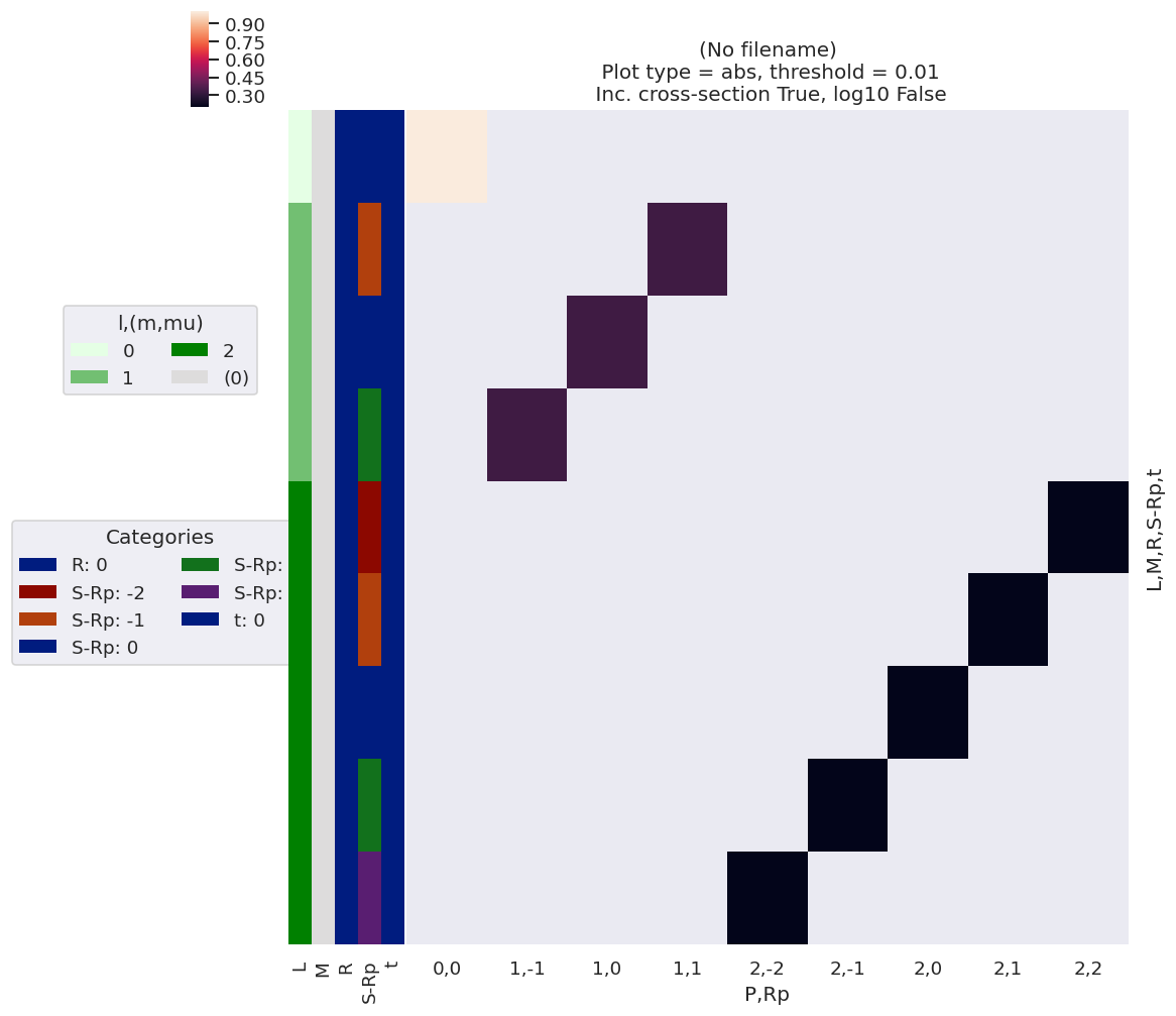
In this case, we could also compose the density matrix directly by passing the relevant dims to the plotting function (all other dims will be stacked)…
(Two issues - plotting may be slow for multi-dim case, and many combinations may be zero/uninteresting.)
[18]:
# Plot
daIn.name = termName # Set name - note this can't be the same as a dimension!
# hvmap = density.matPlot(daIn.squeeze(), kdims = ['P','Rp'])  # Sum & slice data prior to plot
                                                                    # Note that summation may replace NaNs with zeros.
hvmap = density.matPlot(daIn, kdims = ['R','Rp'])
hvmap
WARNING:param.HeatMapPlot264200: Due to internal constraints, when aspect and width/height is set, the bokeh backend uses those values as frame_width/frame_height instead. This ensures the aspect is respected, but means that the plot might be slightly larger than anticipated. Set the frame_width/frame_height explicitly to suppress this warning.
[18]:
[19]:
# Compose density matrix

termName = 'lambdaTerm'  # 'AKQS' # Also needs fixing for single-value case?   # 'lambdaTerm'  # Needs fixing for singleton dim case!  # NOW OK if squeeze = False
daIn = basis[termName]  # Set data

# Set dimensions/state vector/representation
# These must be in original data, but will be restacked as necessary to define the effective basis space.
denDims = ['mu','mup']   # 'ADM'  #
daIn.name = termName

# Calculate + sum over other terms
daOut, *_ = density.densityCalc(daIn, denDims = denDims, selDims = selDims, thres = thres)  #, squeeze = False)  #, sumDims=True)  # OK

daOut.name = termName # Set name - note this can't be the same as a dimension!

# Plot
hvmap = density.matPlot(daOut)  # Sum & slice data prior to plot
                                                                    # Note that summation may replace NaNs with zeros.
hvmap
WARNING:param.HeatMapPlot424103: Due to internal constraints, when aspect and width/height is set, the bokeh backend uses those values as frame_width/frame_height instead. This ensures the aspect is respected, but means that the plot might be slightly larger than anticipated. Set the frame_width/frame_height explicitly to suppress this warning.
Set plot kdims to ['mu,mup', 'mu,mup_p']; pass kdims = [dim1,dim2] for more control.
[19]:
[20]:
ep.util.misc.checkDims(daIn, refDims = denDims)
[20]:
{'dataDims': ('Rp', 'P', 'mu', 'mup', 'Labels'),
 'dataDimsUS': ('Rp', 'P', 'mu', 'mup', 'Labels'),
 'refDims': ['mu', 'mup'],
 'refDimsUS': ['mu', 'mup'],
 'shared': ['mu', 'mup'],
 'extra': ['Labels', 'Rp', 'P'],
 'extraUS': [],
 'invalid': [],
 'invalidUS': [],
 'stacked': [],
 'stackedMap': {},
 'stackedShared': [],
 'stackedExtra': [],
 'stackedComponents': [],
 'stackedInvalid': [],
 'missing': [],
 'safeStack': {},
 'stackedRef': False,
 'nonDimCoords': ['Euler'],
 'nonDimMap': {},
 'nonDimStacked': {},
 'nonDimDicts': {},
 'nonDimDims': {}}
Density matrix from geometric tensors
As discussed here, photoionization can be defined in terms of a set of geometric tensors (state multipoles). These are intimately related to the density matrix, and can be thought of as a coupled basis equivalent.
For example, in the \(\{|JM\rangle\}\) representation (Eqn. 4.8 in Blum [1]):
\begin{equation} \hat{T}(J',J)_{KQ}=\sum_{M'M}(-1)^{J'-M'}(2K+1)^{1/2}\left(\begin{array}{ccc} J' & J & K\\ M' & -M & Q \end{array}\right)|J'M'\rangle\langle JM| \end{equation}
Where \(\hat{T}(J',J)_{KQ}\) are tensor operators. The corresponding matrix elements are (Eqn. 4.9 in Blum [1]):
\begin{equation} \langle J'M'|\hat{T}(J',J)_{KQ}|JM\rangle=(-1)^{J'-M'}(2K+1)^{1/2}\left(\begin{array}{ccc} J' & J & K\\ M' & -M & Q \end{array}\right) \end{equation}
The density matrix can be written in terms of the tensor operators (Eqn. 4.30 in Blum):
\begin{equation} \boldsymbol{\rho}=\sum_{KQ}\sum_{J'J}\left[\sum_{M'M}\langle J'M'|\hat{\rho}|JM\rangle(-1)^{J'-M'}(2K+1)^{1/2}\left(\begin{array}{ccc} J' & J & K\\ M' & -M & Q \end{array}\right)\right]\hat{T}(J',J)_{KQ} \end{equation}
And the state multipoles are defined as the term in square brackets (Eqn. 4.31 in Blum):
\begin{equation} \left\langle T(J',J)_{KQ}^{\dagger}\right\rangle =\sum_{M'M}\langle J'M'|\hat{\rho}|JM\rangle(-1)^{J'-M'}(2K+1)^{1/2}\left(\begin{array}{ccc} J' & J & K\\ M' & -M & -Q \end{array}\right) \end{equation}
And the inverse (Eqn. 4.34 in Blum):
\begin{equation} \langle J'M'|\hat{\rho}|JM\rangle=\sum_{KQ}(-1)^{J'-M'}(2K+1)^{1/2}\left(\begin{array}{ccc} J' & J & K\\ M' & -M & -Q \end{array}\right)\left\langle T(J',J)_{KQ}^{\dagger}\right\rangle \end{equation}
As discussed above, the AF-\(\beta_{LM}\) routines currently define a set of geometric tensors. These can be regarded & treated in general as state multipole type terms (although this is not strictly true in all cases) with appropriate summations. This means that the basis can be readily expressed in terms of mulitpoles or density matrices, and a few examples are given below.
(Note demos in previous section only plot existing tensors, but don’t convert definitions.)
TODO: update matPlot & consolidate dim-handling routines from densityCalc to provide easier plotting routines here (without manual restack etc.).
Density matrix from arb tensors
As of commit e2dcdd326e6e144fb4c442383ee096353314b17f (23/07/24), densityFromSphTensor() is available. This implements the final equation above (Eqn. 4.34 in Blum) to convert an input spherical tensor to density matrix form.
[21]:
# Create arb time-dependent tensor using `setBLMs`
from epsproc.sphCalc import setBLMs
TKQ = setBLMs([[0,0,1,1,1,1,1,1],
               [1,0,0,0.5,0.8,1,0.5,0],[1,-1,0,0.5,0.8,1,0.5,0],[1,1,0,0.5,-0.5,1,0.5,0],
               [2,0,1,0.5,0,0,0.5,1],
               [4,2,0,0,0,0.5,0.8,1],[4,-2,0,0,0,0,-0.8,1]])
               # LMlabels = ['K','Q'], dimNames = ['KQ','t'])

# Rename dims to match arb case...
TKQ = TKQ.unstack('BLM').rename({'l':'K','m':'Q'}).stack({'KQ':['K','Q']})  #.fillna(0)  # Optional
TKQ.attrs['dataType']='TKQ'

# Compute density matrix
# Default case should work for preset datatypes, or pass dims for more control.
# Other dims should be handled/propagated transparently.
pmmFromTKQ = density.densityFromSphTensor(TKQ)

# Full results as Xarray, note default case may also keep input sph tensor dims, which should be summed over for the standard result.
pmmFromTKQ = pmmFromTKQ.sum(['K','Q'])
pmmFromTKQ
Set denDims={'JM': ['J', 'M'], 'JpMp': ['Jp', 'Mp']}. Pass directly for more control.
Set sphDims={'KQ': ['K', 'Q']}. Pass directly for more control.
['J', 'Jp']
['M', 'Mp']
['J', 'Jp', 'K', 'M', 'Mp', 'Q']
[21]:
<xarray.DataArray 'BLM' (t: 6, JM: 45, JpMp: 45)>
array([[[0., 0., 0., ..., 0., 0., 0.],
        [0., 0., 0., ..., 0., 0., 0.],
        [0., 0., 0., ..., 0., 0., 0.],
        ...,
        [0., 0., 0., ..., 0., 0., 0.],
        [0., 0., 0., ..., 0., 0., 0.],
        [0., 0., 0., ..., 0., 0., 0.]],

       [[0., 0., 0., ..., 0., 0., 0.],
        [0., 0., 0., ..., 0., 0., 0.],
        [0., 0., 0., ..., 0., 0., 0.],
        ...,
        [0., 0., 0., ..., 0., 0., 0.],
        [0., 0., 0., ..., 0., 0., 0.],
        [0., 0., 0., ..., 0., 0., 0.]],

       [[0., 0., 0., ..., 0., 0., 0.],
        [0., 0., 0., ..., 0., 0., 0.],
        [0., 0., 0., ..., 0., 0., 0.],
        ...,
...
        ...,
        [0., 0., 0., ..., 0., 0., 0.],
        [0., 0., 0., ..., 0., 0., 0.],
        [0., 0., 0., ..., 0., 0., 0.]],

       [[0., 0., 0., ..., 0., 0., 0.],
        [0., 0., 0., ..., 0., 0., 0.],
        [0., 0., 0., ..., 0., 0., 0.],
        ...,
        [0., 0., 0., ..., 0., 0., 0.],
        [0., 0., 0., ..., 0., 0., 0.],
        [0., 0., 0., ..., 0., 0., 0.]],

       [[0., 0., 0., ..., 0., 0., 0.],
        [0., 0., 0., ..., 0., 0., 0.],
        [0., 0., 0., ..., 0., 0., 0.],
        ...,
        [0., 0., 0., ..., 0., 0., 0.],
        [0., 0., 0., ..., 0., 0., 0.],
        [0., 0., 0., ..., 0., 0., 0.]]])
Coordinates:
  * t        (t) int64 0 1 2 3 4 5
  * JM       (JM) MultiIndex
  - J        (JM) int64 0 0 0 0 0 0 0 0 0 1 1 1 1 ... 3 3 3 3 4 4 4 4 4 4 4 4 4
  - M        (JM) int64 4 3 2 1 0 -1 -2 -3 -4 4 3 ... -4 4 3 2 1 0 -1 -2 -3 -4
  * JpMp     (JpMp) MultiIndex
  - Jp       (JpMp) int64 0 0 0 0 0 0 0 0 0 1 1 1 1 ... 3 3 3 4 4 4 4 4 4 4 4 4
- Mp (JpMp) int64 -4 -3 -2 -1 0 1 2 3 4 -4 ... 4 -4 -3 -2 -1 0 1 2 3 4[22]:
# from epsproc.sphFuncs.sphConv import cleanLMcoords
# # cleanLMcoords(pmmFromTKQ.sel(J=2,Jp=2).stack({'KQ': ['K', 'Q']}), refDims = ['K','Q'])
# pmmFromTKQ.sel(J=2,Jp=2)  #.stack({'KQ': ['K', 'Q']})
[23]:
# Plot, optionally subselect and stack on dims (otherwise all dims will be available in widget)

# density.matPlot(pmmFromTKQ, kdims=['JM','JpMp'])   # All dims

density.matPlot(pmmFromTKQ.sel(J=2,Jp=2))  # With selected J,Jp

# density.matPlot(pmmFromTKQ.sel(J=2,Jp=2).stack({'KQ': ['K', 'Q']}), kdims=['M','Mp'])  # Select on J,Jp and restack sphDims for unsummed case
Set plot kdims to ['M', 'Mp']; pass kdims = [dim1,dim2] for more control.
WARNING:param.HeatMapPlot431177: Due to internal constraints, when aspect and width/height is set, the bokeh backend uses those values as frame_width/frame_height instead. This ensures the aspect is respected, but means that the plot might be slightly larger than anticipated. Set the frame_width/frame_height explicitly to suppress this warning.
[23]:
\(B_{L,M}\) term
The coupling of the partial wave pairs, \(|l,m\rangle\) and \(|l',m'\rangle\), into the observable set of \(\{L,M\}\) is defined by a tensor contraction with two 3j terms.
\begin{equation} B_{L,M}=(-1)^{m}\left(\frac{(2l+1)(2l'+1)(2L+1)}{4\pi}\right)^{1/2}\left(\begin{array}{ccc} l & l' & L\\ 0 & 0 & 0 \end{array}\right)\left(\begin{array}{ccc} l & l' & L\\ -m & m' & M \end{array}\right) \end{equation}
Note for the AF case \(B_{L,S-R'}(l,l',m,m')\) instead of \(B_{L,-M}(l,l',m,m')\) for MF case. This allows for all MF projections to contribute (rather than a single specified polarization geometry).
This term, with a subset of elements defined for the photoionization matrix elements set previously, is (currently, v1.3.0) given by the ‘BLMtableResort’ basis array.
[24]:
basis['BLMtableResort']
[24]:
<xarray.DataArray 'w3jStacked' (m: 3, mp: 3, S-Rp: 5, l: 4, lp: 4, L: 8)>
array([[[[[[        nan,         nan,         nan, ...,         nan,
                    nan,         nan],
           [        nan,         nan,         nan, ...,         nan,
                    nan,         nan],
           [        nan,         nan,         nan, ...,         nan,
                    nan,         nan],
           [        nan,         nan,         nan, ...,         nan,
                    nan,         nan]],

          [[        nan,         nan,         nan, ...,         nan,
                    nan,         nan],
           [        nan,         nan,         nan, ...,         nan,
                    nan,         nan],
           [        nan,         nan,         nan, ...,         nan,
                    nan,         nan],
           [        nan,         nan,         nan, ...,         nan,
                    nan,         nan]],

          [[        nan,         nan,         nan, ...,         nan,
                    nan,         nan],
...
           [        nan,         nan,         nan, ...,         nan,
                    nan,         nan]],

          [[        nan,         nan,         nan, ...,         nan,
                    nan,         nan],
           [        nan,         nan,         nan, ...,         nan,
                    nan,         nan],
           [        nan,         nan,         nan, ...,         nan,
                    nan,         nan],
           [        nan,         nan,         nan, ...,         nan,
                    nan,         nan]]]]]])
Coordinates:
  * L        (L) int64 0 2 4 6 8 10 12 14
  * m        (m) int64 -1 0 1
  * mp       (mp) int64 -1 0 1
  * S-Rp     (S-Rp) int64 -2 -1 0 1 2
  * l        (l) int64 1 3 5 7
  * lp       (lp) int64 1 3 5 7
Attributes:
    dataType:   betaTerm
phaseCons: {'phaseConvention': 'E', 'genMatEcons': {'negm': False}, 'EPR...The lmPlot() routine can be used to show the full dimensionality…
[25]:
# Plot BLM term with restack to standard LM terms
ep.lmPlot(basis['BLMtableResort'].rename({'S-Rp':'M'}).stack({'LM':['L','M']}), xDim={'LM':['L','M']});
Plotting data (No filename), pType=a, thres=0.01, with Seaborn
No artists with labels found to put in legend. Note that artists whose label start with an underscore are ignored when legend() is called with no argument.
The above shows, essentially, all the terms in the summation. By suitable summation we can look at the corresponding density matrix or state multipole.
[26]:
# Compose density matrix

termName = 'BLMtableResort'  # 'AKQS' # Also needs fixing for single-value case?   # 'lambdaTerm'  # Needs fixing for singleton dim case!  # NOW OK if squeeze = False
daIn = basis[termName]  # Set data

# Reformat
daIn = daIn.rename({'S-Rp':'M'}).stack({'LM':['L','M'], 'lm':['l','m'], 'lmp':['lp','mp']})

# Set dimensions/state vector/representation
# These must be in original data, but will be restacked as necessary to define the effective basis space.
denDims = ['lm','lmp']   # 'ADM'  #
daIn.name = termName

hvmap = density.matPlot(daIn.sum('LM').squeeze(), kdims = denDims)

hvmap
WARNING:param.HeatMapPlot434377: Due to internal constraints, when aspect and width/height is set, the bokeh backend uses those values as frame_width/frame_height instead. This ensures the aspect is respected, but means that the plot might be slightly larger than anticipated. Set the frame_width/frame_height explicitly to suppress this warning.
[26]:
[27]:
# Plot tensor BLM (state multipole) term with restack to standard LM terms
hvmap = density.matPlot(daIn.sum(['lm','lmp']).unstack(), kdims = ['L','M'])
hvmap
WARNING:param.HeatMapPlot434538: Due to internal constraints, when aspect and width/height is set, the bokeh backend uses those values as frame_width/frame_height instead. This ensures the aspect is respected, but means that the plot might be slightly larger than anticipated. Set the frame_width/frame_height explicitly to suppress this warning.
[27]:
Lambda terms
[28]:
# Compose density matrix

termName = 'lambdaTerm'  # 'AKQS' # Also needs fixing for single-value case?   # 'lambdaTerm'  # Needs fixing for singleton dim case!  # NOW OK if squeeze = False
daIn = basis[termName]  # Set data

# Set dimensions/state vector/representation
# These must be in original data, but will be restacked as necessary to define the effective basis space.
denDims = ['mu','mup']   # 'ADM'  #
daIn.name = termName

hvmap = density.matPlot(daIn.squeeze(), kdims = denDims)
[29]:
hvmap
WARNING:param.HeatMapPlot435058: Due to internal constraints, when aspect and width/height is set, the bokeh backend uses those values as frame_width/frame_height instead. This ensures the aspect is respected, but means that the plot might be slightly larger than anticipated. Set the frame_width/frame_height explicitly to suppress this warning.
[29]:
[30]:
# Try with explicity summation over tensor (K,Q) dims...
# hvmap = density.matPlot(daIn.sum(['P','Rp']).squeeze(), kdims = denDims)  # Sum over P,Rp
hvmap = density.matPlot(daIn.sum('Rp').squeeze(), kdims = denDims)  # Sum over Rp only
hvmap.layout('P').cols(1)
WARNING:param.HeatMapPlot454337: Due to internal constraints, when aspect and width/height is set, the bokeh backend uses those values as frame_width/frame_height instead. This ensures the aspect is respected, but means that the plot might be slightly larger than anticipated. Set the frame_width/frame_height explicitly to suppress this warning.
WARNING:param.HeatMapPlot454342: Due to internal constraints, when aspect and width/height is set, the bokeh backend uses those values as frame_width/frame_height instead. This ensures the aspect is respected, but means that the plot might be slightly larger than anticipated. Set the frame_width/frame_height explicitly to suppress this warning.
WARNING:param.HeatMapPlot454347: Due to internal constraints, when aspect and width/height is set, the bokeh backend uses those values as frame_width/frame_height instead. This ensures the aspect is respected, but means that the plot might be slightly larger than anticipated. Set the frame_width/frame_height explicitly to suppress this warning.
[30]:
[31]:
# Full response function
# TODO: restacking + summation routine for general cases like this (with multiple existing dims).
basis['BLMtableResort'] * basis['polProd']
[31]:
<xarray.DataArray (m: 3, mp: 3, S-Rp: 5, l: 4, lp: 4, L: 2, mu: 3, mup: 3,
                   Labels: 1, M: 1, t: 1)>
array([[[[[[[[[[[        nan+nanj]]],


              [[[        nan+nanj]]],


              [[[        nan+nanj]]]],


             [[[[        nan+nanj]]],


              [[[        nan+nanj]]],


              [[[        nan+nanj]]]],


...


             [[[[        nan+nanj]]],


              [[[        nan+nanj]]],


              [[[        nan+nanj]]]],


             [[[[        nan+nanj]]],


              [[[        nan+nanj]]],


              [[[        nan+nanj]]]]]]]]]]])
Coordinates:
  * L        (L) int64 0 2
  * m        (m) int64 -1 0 1
  * mp       (mp) int64 -1 0 1
  * S-Rp     (S-Rp) int64 -2 -1 0 1 2
  * l        (l) int64 1 3 5 7
  * lp       (lp) int64 1 3 5 7
  * mu       (mu) int64 -1 0 1
  * mup      (mup) int64 -1 0 1
    Euler    (Labels) object (0.0, 0.0, 0.0)
  * Labels   (Labels) <U1 'z'
  * M        (M) int64 0
* t (t) int64 0Versions
[32]:
import scooby
scooby.Report(additional=['epsproc', 'holoviews', 'hvplot', 'xarray', 'matplotlib', 'bokeh'])
[32]:
| Thu Jul 25 09:44:53 2024 EDT | |||||||
| OS | Linux | CPU(s) | 64 | Machine | x86_64 | Architecture | 64bit |
| RAM | 62.8 GiB | Environment | Jupyter | File system | btrfs | ||
| Python 3.10.11 | packaged by conda-forge | (main, May 10 2023, 18:58:44) [GCC 11.3.0] | |||||||
| epsproc | 1.3.2-dev | holoviews | 1.16.2 | hvplot | 0.8.4 | xarray | 2022.3.0 |
| matplotlib | 3.5.3 | bokeh | 3.1.1 | numpy | 1.23.5 | scipy | 1.10.1 |
| IPython | 8.13.2 | scooby | 0.7.2 | ||||
[33]:
# Check current Git commit for local ePSproc version
from pathlib import Path
!git -C {Path(ep.__file__).parent} branch
!git -C {Path(ep.__file__).parent} log --format="%H" -n 1
* 3d-AFPAD-dev
  dev
  master
ba3d6780d95999e518caf85e08e80e7cbc68b6b2
[34]:
# Check current remote commits
!git ls-remote --heads git://github.com/phockett/ePSproc
fatal: unable to connect to github.com:
github.com[0: 140.82.114.4]: errno=Connection timed out
[35]:
!hostname
8fdb9101787f
[36]:
!conda env list
# conda environments:
#
base                  *  /opt/conda
[ ]:
[ ]: