ePolyScat basics tutorial
08/05/20
Paul Hockett
Disclaimer: I am an enthusiastic ePolyScat user for photoionization calculations, but not an expert on the code. Nonetheless, this tutorial aims to go over some of the key features/uses of ePS for such problems - as far as my own usage goes - and provide an introduction and resource to new users.
Overview & resources
- ePolyScat (ePS) is an open-source tool for numerical computation of electron-molecule scattering & photoionization by Lucchese & coworkers. For more details:
- The ePolyScat website and manual. Note that the manual uses a frames-based layout, use the menu on the page to navigate to sub-sections (direct links break the menu).
- Calculation of low-energy elastic cross sections for electron-CF4 scattering, F. A. Gianturco, R. R. Lucchese, and N. Sanna, J. Chem. Phys. 100, 6464 (1994), http://dx.doi.org/10.1063/1.467237
- Cross section and asymmetry parameter calculation for sulfur 1s photoionization of SF6, A. P. P. Natalense and R. R. Lucchese, J. Chem. Phys. 111, 5344 (1999), http://dx.doi.org/10.1063/1.479794
- Applications of the Schwinger variational principle to electron-molecule collisions and molecular photoionization. Lucchese, R. R., Takatsuka, K., & McKoy, V. (1986). Physics Reports, 131(3), 147–221. https://doi.org/10.1016/0370-1573(86)90147-X (comprehensive discussion of the theory and methods underlying the code).
- ePSproc is an open-source tool for post-processing & visualisation of ePS results, aimed primarily at photoionization studies.
- Ongoing documentation is on Read the Docs.
- Source code is available on Github.
- For more background, see the software metapaper for the original release of ePSproc (Aug. 2016): ePSproc: Post-processing suite for ePolyScat electron-molecule scattering calculations, on Authorea or arXiv 1611.04043.
- ePSdata is an open-data/open-science collection of ePS + ePSproc results.
- ePSdata collects ePS datasets, post-processed via ePSproc (Python) in Jupyter notebooks, for a full open-data/open-science transparent pipeline.
- ePSdata is currently (Jan 2020) collecting existing calculations from 2010 - 2019, from the femtolabs at NRC, with one notebook per ePS job.
- In future, ePSdata pages will be automatically generated from ePS jobs (via the ePSman toolset, currently in development), for immediate dissemination to the research community.
- Source notebooks are available on the Github project pages, and notebooks + datasets via Zenodo repositories (one per dataset). Each notebook + dataset is given a Zenodo DOI for full traceability, and notebooks are versioned on Github.
- Note: ePSdata may also be linked or mirrored on the existing ePolyScat Collected Results OSF project, but will effectively supercede those pages.
- All results are released under Creative Commons Attribution-NonCommercial-ShareAlike 4.0 (CC BY-NC-SA 4.0) license, and are part of our ongoing Open Science initiative.
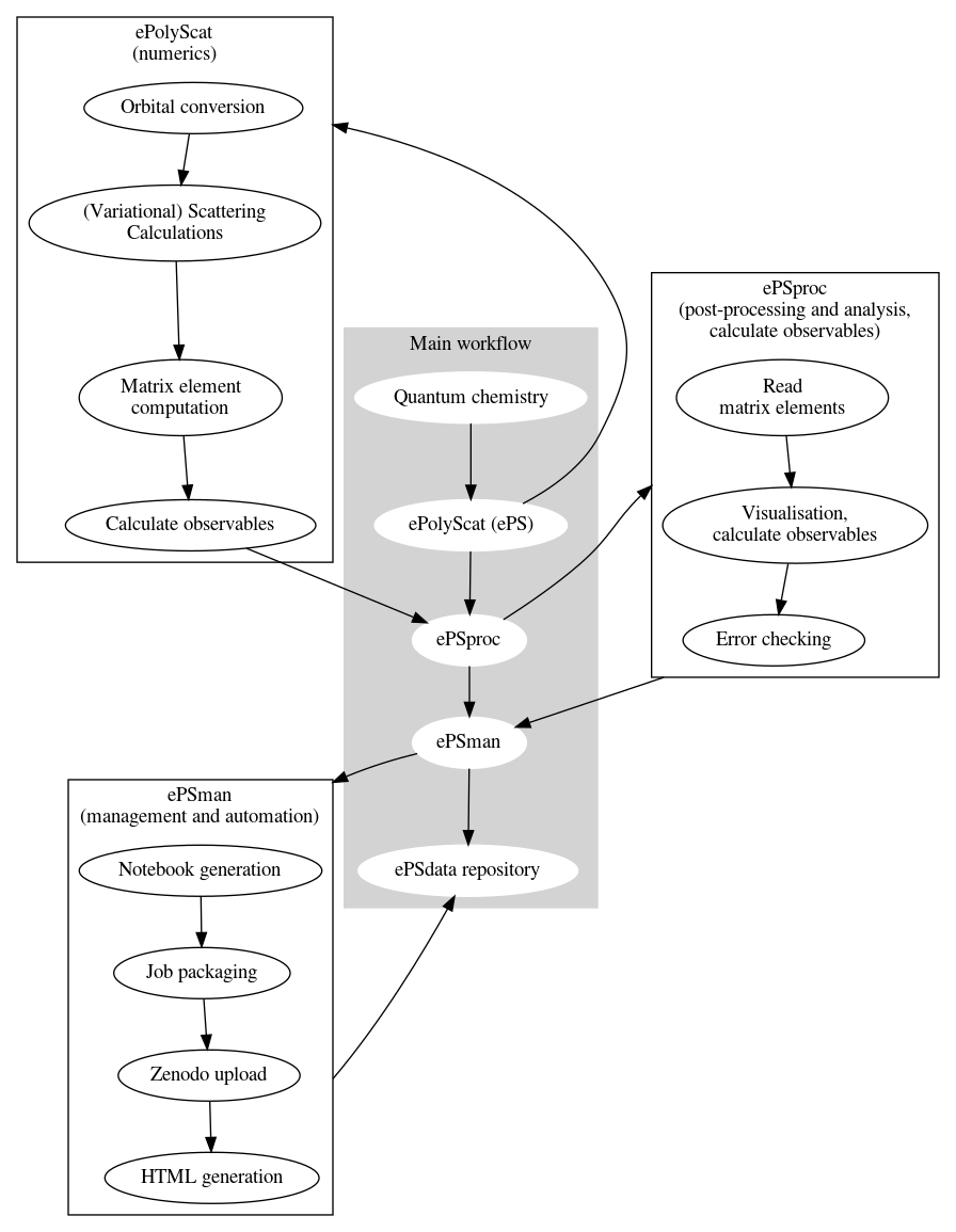
Workflow
The general workflow for photoionization calculations plus post-processing is shown below. This pipeline involves a range of code suites, as shown in the main workflow; some additional details are also illustrated. This tutorial will only discuss ePS.
Theoretical background
For general scattering theory notes, try these textbooks:
- Quantum Mechanics Volume I. Messiah, A. (1970). North-Holland Publishing Company.
- Introduction to the Quantum Theory of Scattering. Rodberg, L. S., & Thaler, R. M. (1967). Academic Press.
For notes focussed on photoionization problems, try:
- Photoelectron angular distributions seminar series
- Brief notes on scattering theory for photoionization
- Quantum Metrology with Photoelectrons, Volume 1 Foundations. Hockett, P. (2018). IOP Publishing. https://doi.org/10.1088/978-1-6817-4684-5
For ePS, the details can be found in:
- Applications of the Schwinger variational principle to electron-molecule collisions and molecular photoionization. Lucchese, R. R., Takatsuka, K., & McKoy, V. (1986). Physics Reports, 131(3), 147–221. https://doi.org/10.1016/0370-1573(86)90147-X (comprehensive discussion of the theory and methods underlying the code).
- Calculation of low-energy elastic cross sections for electron-CF4 scattering, F. A. Gianturco, R. R. Lucchese, and N. Sanna, J. Chem. Phys. 100, 6464 (1994), http://dx.doi.org/10.1063/1.467237
- Cross section and asymmetry parameter calculation for sulfur 1s photoionization of SF6, A. P. P. Natalense and R. R. Lucchese, J. Chem. Phys. 111, 5344 (1999), http://dx.doi.org/10.1063/1.479794
The Method section from the latter paper is reproduced here for reference:
Both the initial neutral molecule electronic wave function and the final ionized molecule electronic wave function are represented by single determinants constructed using the Hartree–Fock orbitals of the initial neutral state. The final \(N\)–electron state (continuum photoelectron + molecular ion) can then be variationally obtained from:
where \(\delta\Psi_{\mathbf{k}}\) represent variations in the final state due to variations on the continuum wave function \(\psi_{\mathbf{k}}(\mathbf{r})\), and \(\mathbf{k}\) is the momentum of the ejected electron. The final photoionization problem is then reduced to solving the problem of an electron under the action of the potential of the ion. Thus, we do not consider many-electron effects. The following scattering equation can be obtained from Eq. (1) (Ref. 19) (in atomic units),
where \(V(\mathbf{r})\) is the static exchange potential given by:
for \(M\) nuclei of charge \(Z_{\gamma}\) located at \(\mathbf{R}\gamma\) , where \(n_{occ}\) is the number of doubly occupied orbitals. \(\hat{J}_{i}\) is the Coulomb operator,
and \(\hat{K}_{i}\) is the nonlocal exchange potential operator
Correlation and polarization effects can be included in the calculations through the addition of a local, energy independent model correlation polarization potential, such as described in Ref. 10 {[}…{]}
To solve the scattering problem, we use the single center expansion (SCE) method, where all three dimensional functions are expanded on a set of angular functions \(X_{lh}^{p\mu}(\theta,\phi)\), which are symmetry adapted, according to the irreducible representations of the molecular point group. An arbitrary three dimensional function \(F^{p\mu}(r,\theta,\phi)\) is then expanded as
where
and \(p\) is one of the irreducible representations of the molecular point group, \(m\) is a component of the representation \(p\), and \(h\) indexes all possible \(X_{lh}^{p\mu}\) belonging to the same irreducible representation (\(p\mu\)) with the same value of \(l\). \emph{The radial functions $f_{lh}^{p\mu}(r)$ are represented on a numerical grid}. When solving the scattering equations we enforce orthogonality between the continuum solutions and the occupied orbitals.\(^{19}\)
The matrix elements of the dipole operator are
for the dipole length form, and
for the dipole velocity form, where \(|\Psi_{i}\rangle\) is the initial bound state, \(|\Psi_{f,\mathbf{k}}^{(-)}\rangle\) is the final continuum state, \(E\) is the photon energy, \(\mathbf{k}\) is the momentum of the photoelectron, and \(\hat{n}\) is the direction of polarization of the light, which is assumed to be linearly polarized.
The matrix elements \(I_{\mathbf{k},\hat{n}}^{(L,V)}\) of Eqs. (8) and (9) can be expanded in terms of the \(X_{lh}^{p\mu}\) functions of Eq. (7) as\(^{14}\)
{[}Note here the final term gives polarization (dipole) terms, with \(l=1\), \(h=v\), corresponding to a photon with one unit of angular momentum and projections \(v=-1,0,1\), correlated with irreducible representations \(p_{v}\mu_{v}\).{]}
The differential cross section is given by
where the asymmetry parameter can be written as\(^{14}\)
and the \((l'lm'm|L'M')\) are the usual Clebsch–Gordan coefficients. The total cross section is
where c is the speed of light.
Numerical background
Numerically, ePS proceeds approximately as in the flow-chart above:
- Molecular structure is parsed from the input quantum chemistry results;
- Various functions process this input, plus additional user commands, to set up the problem (e.g. ionizing orbital selection, symmetry-adapted single point expansion, and subsequent determination of the scattering potential \(V(\mathbf{r})\));
- The scattering solution is determined variationally (i.e. solving \(\langle\delta\Psi_{\mathbf{k}}|H-E|\Psi_{\mathbf{k}}\rangle=0\)) - this is essentially the Schwinger variational method, see ePS references at head of section for further details;
- Various outputs are written to file - some examples are discussed below.
It’s the variational solution for the continuum wavefunction that (usually) takes most of the computational effort, and is the core of an ePS run. This procedure can take anywhere from seconds to minutes to hours for a single point (== single input geometry, energy and symmetry), depending on the problem at hand, and the hardware.
In terms of the code, ePS is written in fortran 90, with MPI for parallelism, and LAPACK and BLAS libraries for numerical routines - see the intro section of the manual for more details.
ePolyScat basic example calculation: N2 \(3\sigma_g^{-1}\) photoionization
ePS uses a similar input format to standard quantum chemistry codes, with a series of data records and commands set by the user for a specific job.
As a basic intro, here is test12 from the ePS sample jobs:
#
# input file for test12
#
# N2 molden SCF, (3-sigma-g)^-1 photoionization
#
  LMax   22     # maximum l to be used for wave functions
  EMax  50.0    # EMax, maximum asymptotic energy in eV
  FegeEng 13.0   # Energy correction (in eV) used in the fege potential

  ScatEng  10.0   # list of scattering energies

 InitSym 'SG'      # Initial state symmetry
 InitSpinDeg 1     # Initial state spin degeneracy
 OrbOccInit 2 2 2 2 2 4  # Orbital occupation of initial state
 OrbOcc     2 2 2 2 1 4  # occupation of the orbital groups of target
 SpinDeg 1         # Spin degeneracy of the total scattering state (=1 singlet)
 TargSym 'SG'      # Symmetry of the target state
 TargSpinDeg 2     # Target spin degeneracy
 IPot 15.581    # ionization potentail

Convert '$pe/tests/test12.molden' 'molden'
GetBlms
ExpOrb

 ScatSym     'SU'  # Scattering symmetry of total final state
 ScatContSym 'SU'  # Scattering symmetry of continuum electron

FileName 'MatrixElements' 'test12SU.idy' 'REWIND'
GenFormPhIon
DipoleOp
GetPot
PhIon
GetCro
#
 ScatSym     'PU'  # Scattering symmetry of total final state
 ScatContSym 'PU'  # Scattering symmetry of continuum electron

FileName 'MatrixElements' 'test12PU.idy' 'REWIND'
GenFormPhIon
DipoleOp
GetPot
PhIon
GetCro
#
GetCro 'test12PU.idy' 'test12SU.idy'
#
#
Let’s breakdown the various segments to this input file…
System & job definition
Basic file header info, comments with #.
#
# input file for test12
#
# N2 molden SCF, (3-sigma-g)^-1 photoionization
#
Defined some numerical values for the calculation - the values here are defined in the Data Records section of the manual, and may have defaults if not set.
LMax   22     # maximum l to be used for wave functions
EMax  50.0    # EMax, maximum asymptotic energy in eV
FegeEng 13.0   # Energy correction (in eV) used in the fege potential

ScatEng  10.0   # list of scattering energies
Define symmetries and orbital occupations. Note that the orbitals are grouped by degeneracy in ePS, so the numbering here may be different from that in the raw computational chemistry file output (which is typically not grouped).
InitSym 'SG'      # Initial state symmetry
InitSpinDeg 1     # Initial state spin degeneracy
OrbOccInit 2 2 2 2 2 4  # Orbital occupation of initial state
OrbOcc     2 2 2 2 1 4  # occupation of the orbital groups of target
SpinDeg 1         # Spin degeneracy of the total scattering state (=1 singlet)
TargSym 'SG'      # Symmetry of the target state
TargSpinDeg 2     # Target spin degeneracy
IPot 15.581    # ionization potentail
Note that the symmetries set here correspond to specific orbital and continuum sets, so there may be multiple symmetries for a given problem - more on this later.
Init job & run calculations
Define electronic structure (in this case, from a Molden file), and run a single-point expansion in symmetry adapted harmonics (see Commands manual pages for more details).
Convert '$pe/tests/test12.molden' 'molden'   # Read electronic structure file
GetBlms
ExpOrb
The meat of ePS is running scattering computations, and calculating associated matrix elements/parameters/observables. In this case, there are two (continuum) symmetries, (SU, PU). In each case, the data records are set, and a sequence of commands run the computations to numerically determine the continuum (scattering) wavefunction (again, more details can be found via the Commands manual pages, comments added below are the basic
command descriptions).
 ScatSym     'SU'  # Scattering symmetry of total final state
 ScatContSym 'SU'  # Scattering symmetry of continuum electron

FileName 'MatrixElements' 'test12SU.idy' 'REWIND'   # Set file for matrix elements
GenFormPhIon   # Generate potential formulas for photoioniztion.
DipoleOp       # Compute the dipole operator onto an orbital.
GetPot         # Calculate electron density, static potential, and V(CP) potential.
PhIon          # Calculate photionization dipole matrix elements.
GetCro         # Compute photoionization cross sections from output of scatstab or from a file of dynamical coefficients.

# Repeat for 2nd symmetry
#
 ScatSym     'PU'  # Scattering symmetry of total final state
 ScatContSym 'PU'  # Scattering symmetry of continuum electron

FileName 'MatrixElements' 'test12PU.idy' 'REWIND'
GenFormPhIon
DipoleOp
GetPot
PhIon
GetCro

# Run a final GetCro command including both symmetries, set by specifying the matrix element files to use.
#
GetCro 'test12PU.idy' 'test12SU.idy'
#
#
Running ePolyScat
Assuming you have ePS compiled/installed, then running the above file is a simple case of passing the file to the ePolyScat executable, e.g. /opt/ePolyScat.E3/bin/ePolyScat inputFile.
For a general code overview see the manual, contact R. R. Lucchese for source code.
Performance will depend on the machine, but for a decent multi-core workstation expect minutes to hours per energy point depending on the size and symmetry of the problem (again, see the test/example jobs for some typical timings.)
Results
Again following quantum chemistry norms, the main output file is an ASCII file with various sections, separated by keyword headers, corresponding different steps in the computations. Additional files - e.g. the matrix elements listed above - may also be of use, although are typically not user-readable/interpretable, but rather provided for internal use (e.g. running further calculations on matrix elements, used with utility programmes, etc.).
The full test12 output file can be found in the manual. We’ll just look at the CrossSection segments, correlated with the GetCro commands in the input, which give the calculated \(\sigma^{L,V}\) and \(\beta_{\mathbf{k}}^{L,V}\) values (as per definitions above).
Here’s the first exampe, for SU symmetry
----------------------------------------------------------------------
CrossSection - compute photoionization cross section
----------------------------------------------------------------------

Ionization potential (IPot) =     15.5810 eV
Label -
Cross section by partial wave      F
Cross Sections for

     Sigma LENGTH   at all energies
      Eng
    25.5810  0.57407014E+01

     Sigma MIXED    at all energies
      Eng
    25.5810  0.53222735E+01

     Sigma VELOCITY at all energies
      Eng
    25.5810  0.49344024E+01

     Beta LENGTH   at all energies
      Eng
    25.5810  0.47433563E+00

     Beta MIXED    at all energies
      Eng
    25.5810  0.47537873E+00

     Beta VELOCITY at all energies
      Eng
    25.5810  0.47642429E+00

          COMPOSITE CROSS SECTIONS AT ALL ENERGIES
         Energy  SIGMA LEN  SIGMA MIX  SIGMA VEL   BETA LEN   BETA MIX   BETA VEL
EPhi     25.5810     5.7407     5.3223     4.9344     0.4743     0.4754     0.4764
Time Now =        19.9228  Delta time =         0.0067 End CrossSection
This provides a listing of the photoionization cross-section(s) \(\sigma\) (in mega barns, 1 Mb = \(10^{-18} cm^2\)), and associated anisotropy parameter(s) \(\beta\) (dimensionless) - in this case, just for a single energy point. Note that there are multiple values, these correspond to calculations in \(L\) or \(V\) gauge. The values are also tabulated at the end of the output, along with a note on the computational time.
Note that these values correspond to calculations for an isotropic ensemble, i.e. what would usually be measured in the lab frame for a 1-photon ionization from a gas sample, as given by the \(\beta_{\mathbf{k}}^{L,V}\) values defined earlier). For these normalised values, the differential cross section (photoelectron flux vs. angle) \(\frac{d\sigma^{L,V}}{d\Omega_{\mathbf{k}}}\) defined earlier can be written in a slightly simplified form, \(I(\theta) = \sigma(1 + \beta \cos^2(\theta))\) (note this is, by definition, cylindrically symmetric).
Here’s the values corresponding to PU symmetry:
----------------------------------------------------------------------
CrossSection - compute photoionization cross section
----------------------------------------------------------------------

Ionization potential (IPot) =     15.5810 eV
Label -
Cross section by partial wave      F
Cross Sections for

     Sigma LENGTH   at all energies
      Eng
    25.5810  0.30571336E+01

     Sigma MIXED    at all energies
      Eng
    25.5810  0.27828683E+01

     Sigma VELOCITY at all energies
      Eng
    25.5810  0.25404131E+01

     Beta LENGTH   at all energies
      Eng
    25.5810  0.12686831E+01

     Beta MIXED    at all energies
      Eng
    25.5810  0.13002321E+01

     Beta VELOCITY at all energies
      Eng
    25.5810  0.13302595E+01

          COMPOSITE CROSS SECTIONS AT ALL ENERGIES
         Energy  SIGMA LEN  SIGMA MIX  SIGMA VEL   BETA LEN   BETA MIX   BETA VEL
EPhi     25.5810     3.0571     2.7829     2.5404     1.2687     1.3002     1.3303
Time Now =        35.0804  Delta time =         0.0067 End CrossSection
… and the final set of values for both continua:
----------------------------------------------------------------------
CrossSection - compute photoionization cross section
----------------------------------------------------------------------

Ionization potential (IPot) =     15.5810 eV
Label -
Cross section by partial wave      F
Cross Sections for

     Sigma LENGTH   at all energies
      Eng
    25.5810  0.87978350E+01

     Sigma MIXED    at all energies
      Eng
    25.5810  0.81051418E+01

     Sigma VELOCITY at all energies
      Eng
    25.5810  0.74748155E+01

     Beta LENGTH   at all energies
      Eng
    25.5810  0.10200847E+01

     Beta MIXED    at all energies
      Eng
    25.5810  0.10432056E+01

     Beta VELOCITY at all energies
      Eng
    25.5810  0.10660644E+01

          COMPOSITE CROSS SECTIONS AT ALL ENERGIES
         Energy  SIGMA LEN  SIGMA MIX  SIGMA VEL   BETA LEN   BETA MIX   BETA VEL
EPhi     25.5810     8.7978     8.1051     7.4748     1.0201     1.0432     1.0661
In this case, the SU continua has a larger XS (~5.7 Mb) and a larger \(\beta\) value, hence will have a more anisotropic angular scattering distribution. The values for the different gauges are similar, indicating that these results should be (numerically) accurate - generally speaking, the differences in results between different gauges can be regarded as indicative of numerical accuracy and stability. (See, for example *Atoms and Molecules in Intense Laser Fields: Gauge Invariance ofTheory and Models*, A. D. Bandrauk, F. Fillion-Gourdeau and E. Lorin, arXiv 1302.2932 (best ref…?).)
ePolyScat: preparing an input file
In most cases, this is relatively simple, assuming that there is a suitable test example to use as a template. A few caveats…
- There are quite a few computational parameters which can, and should, be played with. (I have not done enough of this, to be honest.)
- There are lots of commands which are not really covered in the test examples, so exploring the manual is worthwhile.
- One aspect which is non-trivial is the assignment of correct symmetries. To the best of my knowledge (which doesn’t go very far here), there is no easy way to auto-generate these (although ePS will tell you if you got things wrong…), so maybe this can be considered as the necessary barrier to entry…! Some examples are given below.
(Some autogeneration for input files & general job management is currently in development.)
Symmetry selection rules in photoionization
Essentially, the relevant direct products must contain the totally symmetric representation of the point group to constitute an allowed combination:
Where \(\Gamma\) is the character of the quantity of interest. For the neutral and ion this will be the direct product of unpaired electrons - hence, for a closed-shell system, this is usually totally symmetric for the neutral, and identical to the character of the ionizing orbital for the ion. The dipole character corresponds to the \((x,y,z)\) operators in the point group, and the electron (continuum) character is what one needs to work out.
For more discussion, see, for example, Signorell, R., & Merkt, F. (1997). General symmetry selection rules for the photoionization of polyatomic molecules. Molecular Physics, 92(5), 793–804. DOI: 10.1080/002689797169745
Worked example: N2 \(3\sigma_g^{-1}\)
This corresponds to the test case above. We’ll need the character table for \(D_{\infty h}\) (see also Oxford materials page from Atkins, Child & Philips, which includes the direct product tables (PDF version). Then just plug in and work through…
Hence:
Finally we also need to specify the total scattering symmetry \(\Gamma_{\mathrm{scat}}=\Gamma_{\mathrm{ion}}\otimes\Gamma_{\mathrm{electron}}\):
… which is identical to \(\Gamma_{\mathrm{electron}}\) in this simple case.
These symmetries correspond to the SU and PU cases set in the ePS input earlier. (A full list of ePS supported symmetries is given in the manual.) It is worth noting that the continua correspond to the polarisation of the electric field in the molecular frame, hence which (Cartesian) dipole component is selected.
Example: NO2 with autogeneration
(To follow - part of epsman development…!)
Multi-energy calculations
The most common case (for photoionization problems) is likely to be setting multiple energy points for a calculation. An example is shown in test04 (full output), which basically uses the ScatEng record:
ScatEng 0.5 10.0 15.0 # list of scattering energies
In this case, later use of GetCro will output properties at the energies set here.
ePolyScat: advanced usage
See pt. 2 notebook!
- Working directly with matrix elements.
- Post-processing with ePSproc.