ePSproc wavefunction plotting tests & demo
20/07/20
This notebook demos (continuum photoelectron) wavefunction plotting from ePS gridded file outputs. The plotting is handled with pyVista, with itkwidgets for interactive plotting. Both tools are built on the ITK/VTK toolchain.
Aims:
- Implement wfPlot.py module.
- Test & demo.
See also:
- Early dev notebook, http://localhost:8888/notebooks/github/ePSproc/epsproc/tests/plottingDev/pyVista_tests_070320_basics_working_150320.ipynb
- Extended test notebook: http://localhost:8888/notebooks/github/ePSproc/epsproc/tests/plottingDev/ePSproc_wfPlot_tests_150720.ipynb
- Orbital plotting, https://epsproc.readthedocs.io/en/dev/methods/ePSproc_orbPlot_tests_130520.html
Setup
[1]:
# Standard libs
import sys
import os
from pathlib import Path
import numpy as np
import xarray as xr

from datetime import datetime as dt
timeString = dt.now()

# For reporting
import scooby
# scooby.Report(additional=['holoviews', 'hvplot', 'xarray', 'matplotlib', 'bokeh'])
# TODO: set up function for this, see https://github.com/banesullivan/scooby
[2]:
# Installed package version
# import epsproc as ep

# ePSproc test codebase (local)
if sys.platform == "win32":
    modPath = r'D:\code\github\ePSproc'  # Win test machine
else:
    modPath = r'/home/femtolab/github/ePSproc/'  # Linux test machine

sys.path.append(modPath)
import epsproc as ep
* plotly not found, plotly plots not available.
* pyevtk not found, VTK export not available.
wfPlotter class
This provides a basic interface to pyVista plotting methods. An object is created with the wavefunction data (from file(s)) and set as a pyVista object, .vol, with a set of data arrays.
For testing, there’s a single demo data file in the ePSproc repo, DABCOSA2PPCA2PP_10.5eV_Orb.dat, which is an example wavefunction for DABCO scattering at 10.5eV, \(A_{2}"\) continuum symmetry.
For more general use, an interface to ePSdata and Zenodo is in development.
[3]:
# Load class and data
from epsproc.vol.wfPlot import wfPlotter

# Load data from modPath\data
dataPath = os.path.join(modPath, 'data', 'wavefn')

wfClass = wfPlotter(fileBase = dataPath)
*** Scanning dir
/home/femtolab/github/ePSproc/data/wavefn
Found 1 _Orb.dat file(s)

Read 1 wavefunction data files OK.
*** Grids set OK
*** Data set OK
StructuredGrid (0x7f0d97d33f30)
  N Cells:      129600
  N Points:     137751
  X Bounds:     -1.000e+01, 1.000e+01
  Y Bounds:     -1.000e+01, 1.000e+01
  Z Bounds:     -1.000e+01, 1.000e+01
  Dimensions:   51, 37, 73
  N Arrays:     3
[4]:
# Display pyVista object info
wfClass.vol
[4]:
| Header | Data Arrays | ||||||||||||||||||||||||||||||||||||||||
|---|---|---|---|---|---|---|---|---|---|---|---|---|---|---|---|---|---|---|---|---|---|---|---|---|---|---|---|---|---|---|---|---|---|---|---|---|---|---|---|---|---|
|
|
Note that the data arrays are currently numbered by file input, with Re, Im and Abs values. This might change in the future.
[5]:
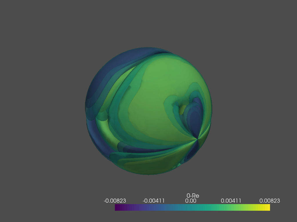
# Plot - default is an interactive version using ITK widgets.
wfClass.plotWf(pType='Re')
wfClass.pl.show()
For HTML output - the interactive widgets (using pv.PlotterITK() and ITK widgets) need a live notebook. For static output, pass interactive=False to the plotter.
[6]:
wfClass.plotWf(pType='Re', interactive=False)
# wfClass.pl.show()
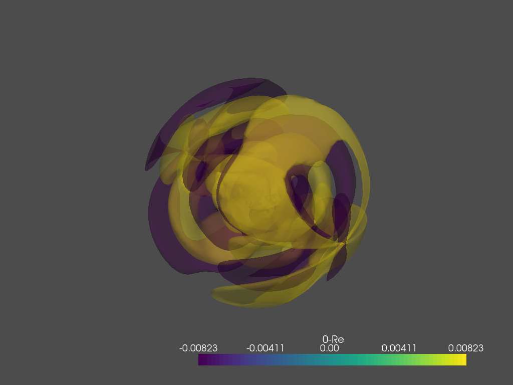
[7]:
# For more control, pass # of iso surfs to plot (default=6), and opacity (default=0.5) (opacity mapping to do!)
wfClass.plotWf(pType='Re', interactive=False, isoLevels=2, opacity=0.3)
# wfClass.pl.show()
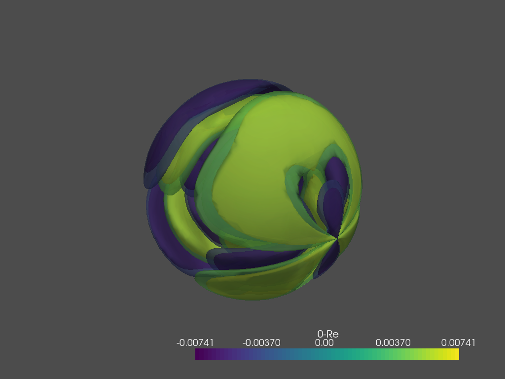
[8]:
# Rather than just specifying a number, isovalues can be passed by %age or absolute value
# NOTE that these are set for +/- pairs, so each value produces two isosurfs (except when plotting the Abs values)

isoValsPC=[0.5,0.9]  # Set isosurfs at 50% and 90% of the max value.
wfClass.plotWf(pType='Re', interactive=False, isoValsPC=isoValsPC)
# wfClass.pl.show()
Versions
[9]:
import scooby
scooby.Report(additional=['epsproc', 'pyvista', 'xarray'])
[9]:
| Tue Jul 21 13:43:58 2020 EDT | |||||
| OS | Linux | CPU(s) | 4 | Machine | x86_64 |
| Architecture | 64bit | RAM | 7.7 GB | Environment | Jupyter |
| Python 3.7.6 (default, Jan 8 2020, 19:59:22) [GCC 7.3.0] | |||||
| epsproc | 1.2.5-dev | pyvista | 0.23.1 | xarray | 0.13.0 |
| numpy | 1.18.1 | scipy | 1.3.1 | IPython | 7.13.0 |
| matplotlib | 3.2.0 | scooby | 0.5.5 | ||
| Intel(R) Math Kernel Library Version 2019.0.4 Product Build 20190411 for Intel(R) 64 architecture applications | |||||