ePSproc wavefunction plotting tests & demo: CH3I with animation¶

11/08/20

This notebook demos (continuum photoelectron) wavefunction plotting from ePS gridded file outputs, for a large dataset including animation. (See the basic notebook for starter demo material.) The plotting is handled with pyVista, with itkwidgets for interactive plotting. Both tools are built on the ITK/VTK toolchain.

Aims:

Test & demo wfPlotter class for large datasets.
Demo animation routine.

Setup¶

[1]:

# Standard libs
import sys
import os
from pathlib import Path
import numpy as np
import xarray as xr

from datetime import datetime as dt
timeString = dt.now()

# For reporting
import scooby
# scooby.Report(additional=['holoviews', 'hvplot', 'xarray', 'matplotlib', 'bokeh'])
# TODO: set up function for this, see https://github.com/banesullivan/scooby

[2]:

# Installed package version
# import epsproc as ep

# ePSproc test codebase (local)
if sys.platform == "win32":
    modPath = r'D:\code\github\ePSproc'  # Win test machine
else:
    modPath = r'/home/femtolab/github/ePSproc/'  # Linux test machine

sys.path.append(modPath)
import epsproc as ep

* pyevtk not found, VTK export not available.

wfPlotter class¶

Data IO and plotting functions are set in the wfPlotter class.

[3]:

from epsproc.vol.wfPlot import wfPlotter

# Load data from modPath\data
# dataPath = os.path.join(modPath, 'data', 'wavefn')  # Case for single test dataset in ePSproc repo

# Load data from an ePSdata download,
# See https://epsproc.readthedocs.io/en/dev/demos/ePSdata_download_demo_300720.html
# dataPath = r'/home/femtolab/Downloads/3660708/CH3I_1-60eV/orb20_A1_waveFn'  # Linux test machine
dataPath = r'D:\temp\3660708\CH3I_1-60eV\orb20_A1_waveFn'   # Win test machine

wfClass = wfPlotter(fileBase = dataPath, tempdir = Path(dataPath).parent)  # Optionally pass tempdir here for output image files (animation only), otherwise will be set to system default.


*** Scanning dir
D:\temp\3660708\CH3I_1-60eV\orb20_A1_waveFn
Found 48 _Orb.dat file(s)

D:\temp\3660708\CH3I_1-60eV\orb20_A1_waveFn\CH3IS
Found molecule: CH3I
Found 2 symmetries, ['SA1CA1', 'SECE']
Found 24 energies, [1.0, 3.5, 6.0, 8.5, 11.0, 13.5, 16.0, 18.5, 21.0, 23.5, 26.0, 28.5, 31.0, 33.5, 36.0, 38.5, 41.0, 43.5, 46.0, 48.5, 51.0, 53.5, 56.0, 58.5]

*** Read existing plot options from file D:\code\github\ePSproc\epsproc\vol\plotOptions.json OK.

File names are stored in .fList This is sorted in “natural” order with the natsort library, or python’s native sorted() function if natsort is not available.

[4]:

wfClass.prefix

[4]:

'D:\\temp\\3660708\\CH3I_1-60eV\\orb20_A1_waveFn\\CH3IS'

[5]:

# First 10 files in the sorted list
wfClass.fList[0:10]

[5]:

['D:\\temp\\3660708\\CH3I_1-60eV\\orb20_A1_waveFn\\CH3ISA1CA1_1.0eV_Orb.dat',
 'D:\\temp\\3660708\\CH3I_1-60eV\\orb20_A1_waveFn\\CH3ISA1CA1_3.5eV_Orb.dat',
 'D:\\temp\\3660708\\CH3I_1-60eV\\orb20_A1_waveFn\\CH3ISA1CA1_6.0eV_Orb.dat',
 'D:\\temp\\3660708\\CH3I_1-60eV\\orb20_A1_waveFn\\CH3ISA1CA1_8.5eV_Orb.dat',
 'D:\\temp\\3660708\\CH3I_1-60eV\\orb20_A1_waveFn\\CH3ISA1CA1_11.0eV_Orb.dat',
 'D:\\temp\\3660708\\CH3I_1-60eV\\orb20_A1_waveFn\\CH3ISA1CA1_13.5eV_Orb.dat',
 'D:\\temp\\3660708\\CH3I_1-60eV\\orb20_A1_waveFn\\CH3ISA1CA1_16.0eV_Orb.dat',
 'D:\\temp\\3660708\\CH3I_1-60eV\\orb20_A1_waveFn\\CH3ISA1CA1_18.5eV_Orb.dat',
 'D:\\temp\\3660708\\CH3I_1-60eV\\orb20_A1_waveFn\\CH3ISA1CA1_21.0eV_Orb.dat',
 'D:\\temp\\3660708\\CH3I_1-60eV\\orb20_A1_waveFn\\CH3ISA1CA1_23.5eV_Orb.dat']

Job details are also extracted from the filenames, and stored in .fDictE (energy sorted) and .fDictSym (symmetry sorted). These are both accessed by simple integer keys.

[6]:

wfClass.fDictE[0]

[6]:

{'E': 1.0,
 'fList': ['D:\\temp\\3660708\\CH3I_1-60eV\\orb20_A1_waveFn\\CH3ISA1CA1_1.0eV_Orb.dat',
  'D:\\temp\\3660708\\CH3I_1-60eV\\orb20_A1_waveFn\\CH3ISECE_1.0eV_Orb.dat'],
 'mol': 'CH3I',
 'syms': ['SA1CA1', 'SECE']}

Select & read files¶

Since there might be quite a bit of data, the files are not read initially. This allows for subselection from the full file list. This can be done via the .selectOrbFiles() method, which will set values for IO, or by passing the selection parameters to the .readOrbFiles() method.

Data dictionaries and subselection¶

Subselection can be made by index value (int), energy value (float) or symmetry group…

[7]:

# The .selectOrbFiles() method is used for selection,
# This is used by .readOrbFiles() below, but can also be called independently (without reading files)

# With ints (index) values
wfClass.selectOrbFiles(EList = [0,5,7])

Selected 3 energies, [1.0, 13.5, 18.5]
Selected symmetries, ['SA1CA1', 'SECE']

[8]:

# With floats, which must correspond to exact values for the data items
wfClass.selectOrbFiles(EList = [8.5,16.0, 16.1])

# Note that unmatched values are ignored here.
# TODO: add a range option and nearest value matching

Selected 2 energies, [8.5, 16.0]
Selected symmetries, ['SA1CA1', 'SECE']

[9]:

# With symmetries
wfClass.selectOrbFiles(SymList = 'SA1CA1')

Selected 24 energies, [1.0, 3.5, 6.0, 8.5, 11.0, 13.5, 16.0, 18.5, 21.0, 23.5, 26.0, 28.5, 31.0, 33.5, 36.0, 38.5, 41.0, 43.5, 46.0, 48.5, 51.0, 53.5, 56.0, 58.5]
Selected symmetries, ['SA1CA1']

[10]:

# With a combination
wfClass.selectOrbFiles(EList = [0,1,6], SymList = 'SA1CA1')

Selected 3 energies, [1.0, 3.5, 16.0]
Selected symmetries, ['SA1CA1']

[11]:

# There's also head & tail methods to check the selected items
wfClass.head()

Item key: 0

[11]:

{'E': 1.0,
 'fList': ['D:\\temp\\3660708\\CH3I_1-60eV\\orb20_A1_waveFn\\CH3ISA1CA1_1.0eV_Orb.dat'],
 'mol': 'CH3I',
 'syms': ['SA1CA1']}

[12]:

wfClass.tail()

Item key: 6

[12]:

{'E': 16.0,
 'fList': ['D:\\temp\\3660708\\CH3I_1-60eV\\orb20_A1_waveFn\\CH3ISA1CA1_16.0eV_Orb.dat'],
 'mol': 'CH3I',
 'syms': ['SA1CA1']}

File IO¶

This is handled by .readOrbFiles(). If a subselection has already been set, it will be used by default, otherwise all files will be read. Selections can also be made as above, plus the additional option of passing a file list directly.

[13]:

# Default case - here the previous selection is used.
wfClass.readOrbFiles()


Read 3 wavefunction data files OK.
*** Grids set OK
*** Data set OK

[14]:

# Set which files should be read, can pass a list of paths here, or index into .fList with ints.
# Note that, in this case, the original fList is reused, and items are resorted, so may not match self.fDictE or self.fDictSym
subSet = [0,5,10,15]
wfClass.readOrbFiles(fList=subSet)

D:\temp\3660708\CH3I_1-60eV\orb20_A1_waveFn\CH3IS
Selected 4 energies, [1.0, 13.5, 26.0, 38.5]
Selected symmetries, ['SA1CA1']

Read 4 wavefunction data files OK.
*** Grids set OK
*** Data set OK

[15]:

# The data items previously set now have all the data appended.
# This is set as a PyVista object in the 'vol' dictionary item
wfClass.head()['vol']

# NOTE - PyVista items are indexed sequentially, so may not match input dict keys. This may change in future.

Item key: 0

[15]:

Header

Data Arrays

StructuredGrid	Information
N Cells	129600
N Points	137751
X Bounds	-1.000e+01, 1.000e+01
Y Bounds	-1.000e+01, 1.000e+01
Z Bounds	-1.000e+01, 1.000e+01
Dimensions	51, 37, 73
N Arrays	3

Name	Field	Type	N Comp	Min	Max
0_E1.0_SA1CA1-Re	Points	float64	1	-2.620e-02	3.391e-02
0_E1.0_SA1CA1-Im	Points	float64	1	-1.611e-01	1.245e-01
0_E1.0_SA1CA1-Abs	Points	float64	1	4.987e-13	2.710e-02

[16]:

wfClass.tail()['vol']

Item key: 3

[16]:

Header

Data Arrays

StructuredGrid	Information
N Cells	129600
N Points	137751
X Bounds	-1.000e+01, 1.000e+01
Y Bounds	-1.000e+01, 1.000e+01
Z Bounds	-1.000e+01, 1.000e+01
Dimensions	51, 37, 73
N Arrays	3

Name	Field	Type	N Comp	Min	Max
3_E38.5_SA1CA1-Re	Points	float64	1	-7.749e-02	9.032e-02
3_E38.5_SA1CA1-Im	Points	float64	1	-4.745e-01	5.530e-01
3_E38.5_SA1CA1-Abs	Points	float64	1	1.569e-15	3.140e-01

Plot¶

The default plot is interactive (with VTK), and will show all the loaded datasets (with given type). Rotation, visibilities and opacities of each plotted dataset can be changed via the menu in the plot window. This is good for initial data exploration. Note, however, that this needs a live notebook process, and won’t render in static HTML output.

[17]:

wfClass.plotWf(pType='Re', opacity=0.3)

Set plotter to PlotterITK

Subplots¶

For non-interactive data exploration, subplots can be used.

[18]:

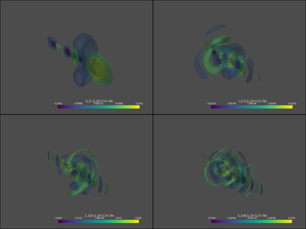
wfClass.plotOptions['global']['subplot'] = True
wfClass.plotWf(pType='Abs')

Set plotter to Plotter

../_images/demos_ePSproc_wfPlot_tests_150720-110820-CH3I-tidy_Stimpy_28_1.png

Animation¶

Multiple frame output and gif generation is (just about) supported.

TODO:

fix global colormap
more annotations
frame rate
fix global (x,y,z) scaling (default crops to contours)

[19]:

wfClass.plotOptions['global']['subplot'] = False
wfClass.plotOptions['global']['animate'] = True

[20]:

wfClass.plotWf(pType='Abs')

Frame images output to:  D:\temp\3660708\CH3I_1-60eV\wfAnimation_CH3I_27-08-20_09-52-41
GIF animation file:  D:\temp\3660708\CH3I_1-60eV\wfAnimation_CH3I_27-08-20_09-52-41\wfAnimation_CH3I_27-08-20_09-52-41.gif
Set plotter to Plotter
Animation output complete.

[20]:

[21]:

wfClass.mol

[21]:

'CH3I'

[22]:

# To get the file path
wfClass.gifFile

[22]:

WindowsPath('D:/temp/3660708/CH3I_1-60eV/wfAnimation_CH3I_27-08-20_09-52-41/wfAnimation_CH3I_27-08-20_09-52-41.gif')

[23]:

# To show the gif
wfClass.showGif()

[23]:

With full E set¶

[24]:

# Set symmetry, all E
wfClass.selectOrbFiles(SymList = 'SA1CA1')
wfClass.readOrbFiles()

Selected 24 energies, [1.0, 3.5, 6.0, 8.5, 11.0, 13.5, 16.0, 18.5, 21.0, 23.5, 26.0, 28.5, 31.0, 33.5, 36.0, 38.5, 41.0, 43.5, 46.0, 48.5, 51.0, 53.5, 56.0, 58.5]
Selected symmetries, ['SA1CA1']

Read 24 wavefunction data files OK.
*** Grids set OK
*** Data set OK

[25]:

wfClass.plotWf(pType='Abs')

Frame images output to:  D:\temp\3660708\CH3I_1-60eV\wfAnimation_CH3I_27-08-20_09-52-57
GIF animation file:  D:\temp\3660708\CH3I_1-60eV\wfAnimation_CH3I_27-08-20_09-52-57\wfAnimation_CH3I_27-08-20_09-52-57.gif
Set plotter to Plotter
Animation output complete.

[25]:

Plot options¶

The default plot options are set in a dictionary. Some options can also be passed directly to the plotter. Currently the defaults are initially read from file, and custom options files can also be used.

TODO:

more options to set, including plotter-specific cases.
general set functionality, rather than manual assignment.

[26]:

# Currently set plotOptions
wfClass.plotOptions

[26]:

{'global': {'note': 'Global plot settings, used as defaults. To change for session, overwrite in local dict. To change permanently, overwrite in file plotOptions.json. To reset, use `epsproc/vol/set_plot_options_json.ipynb` or .py.',
  'pType': 'Abs',
  'interactive': False,
  'inline': True,
  'animate': True,
  'isoLevels': 6,
  'isoValsAbs': None,
  'isoValsPC': None,
  'isoValsGlobal': True,
  'opacity': 0.3,
  'subplot': False},
 'BGplotter': {'addAxis': True, 'kwargs': {}}}

[27]:

# Reset local values from file
wfClass.setPlotOptions()

Overwrite local plot options with settings from file (y/n)?  y


*** Read existing plot options from file D:\code\github\ePSproc\epsproc\vol\plotOptions.json OK.

[28]:

# Setting local options to follow!
wfClass.setPlotOptions(subplot=True)

Arb option setting not yet supported, but can be manually assigned to self.plotOptions dictionary.

[29]:

# Manual assignment to nested dictionary
wfClass.plotOptions['global']['opacity'] = 0.5

wfClass.plotOptions['global']['opacity']

[29]:

0.5

Versions¶

[30]:

import scooby
scooby.Report(additional=['epsproc', 'pyvista', 'xarray'])

[30]:

Thu Aug 27 09:59:04 2020 Eastern Daylight Time
OS	Windows	CPU(s)	32	Machine	AMD64
Architecture	64bit	RAM	63.9 GB	Environment	Jupyter
Python 3.7.3 (default, Apr 24 2019, 15:29:51) [MSC v.1915 64 bit (AMD64)]
epsproc	1.2.5-dev	pyvista	0.25.3	xarray	0.15.0
numpy	1.19.1	scipy	1.3.0	IPython	7.12.0
matplotlib	3.3.1	scooby	0.5.6
Intel(R) Math Kernel Library Version 2020.0.0 Product Build 20191125 for Intel(R) 64 architecture applications