Welcome to ePSproc
ePSproc Readme
Post-processing suite for ePolyScat calculations.
ePSproc scripts are designed for photoionization studies. The scripts were originally written for Matlab (2009 - 2016); a Python version is currently under (heavy) development (Aug. 2019), and will be the main version in future.
Source code is available on Github.
Ongoing documentation is on Read the Docs.
For more background, and details on the Matlab version, see the software metapaper for ePSproc (Aug. 2016), ePSproc: Post-processing suite for ePolyScat electron-molecule scattering calculations, on Authorea or arXiv 1611.04043.
Installation
From source: simply download from Github. See specific version notes below for more details on the source code.
Python:
$ pip install ePSproc
Main requirements are Xarray (>= 0.12.2), and Moble’s spherical functions (quaternion based) (tested with v2019.7.12.23.25.11). See the individual package docs for full instructions - one option is via conda-forge: (Update Sept. 2019 - Xarray v0.13.0 is now on the main Anaconda channel.)
.. $ conda install -c conda-forge xarray=0.12.3
$ conda install -c conda-forge spherical_functions
The usual SciPy stack is also used (numpy, matplotlib etc.) - see requirements.txt for full list - plus some optional packages for additional functionality.
Python
Functionality:
- Read raw photoionization matrix elements from ePS output files with “dumpIdy” segments
- Calculate MF-PADs from the matrix elements (ePSproc_MFPAD.m, see also ePSproc_NO2_MFPADs_demo.m)
- Plot MF-PADs
- Calculate MF-$beta_{LM}$ parameters
- Distirbution via PyPi (latest stable version) .`
- Under development: additional functionality and distribution via PyPi.
See the demo Jupyter notebooks for example usage:
Source:
- ./epsproc: basic python version, code still under development.
- ./docs: documentation tree, HTML version on Read the Docs.
Matlab
Functionality:
- Read raw photoionization matrix elements from ePS output files with “dumpIdy” segments
- Calculate MF-PADs from the matrix elements (ePSproc_MFPAD.m, see also ePSproc_NO2_MFPADs_demo.m)
- Plot MF-PADs
- Plot X-sects
- (Beta testing): Calculate MF-BLMs from matrix elements, see ePSproc_MFBLM.m
- (Under development): Calculate AF-BLMs from matrix elements.
Source:
- /matlab: stable matlab code (as per release v1.0.1).
- a set of functions for processing (ePSproc*.m files)
- a script showing demo calculations, ePSproc_NO2_MFPADs_demo.m
- /docs/additional contains:
- the benchmark results from these calculations, ePSproc_NO2_testing_summary_250915.pdf
- additional notes on ePS photoionization matrix elements, ePSproc_scattering_theory_ePS_notes_011015.pdf.
See ePSproc: Post-processing suite for ePolyScat electron-molecule scattering calculations for more details.
Resources
An ongoing repository of ePS results can be found on OSF.
ePolyScat
For details about ePolyScat (ePS), a tool for computation of electron-molecule scattering, see:
- ePS website & manual, maintained by R.R. Lucchese.
- Calculation of low-energy elastic cross sections for electron-CF4 scattering, F. A. Gianturco, R. R. Lucchese, and N. Sanna, J. Chem. Phys. 100, 6464 (1994), http://dx.doi.org/10.1063/1.467237
- Cross section and asymmetry parameter calculation for sulfur 1s photoionization of SF6, A. P. P. Natalense and R. R. Lucchese, J. Chem. Phys. 111, 5344 (1999), http://dx.doi.org/10.1063/1.479794
Future aims
- Add capabilities, including more general processing, and for other phenomena (e.g. recombination matrix elements for high-harmonic generation, aligned-frame calculations)
- Tidy and streamline code (yep)
- Extend & update notes and benchmark calculations
- Port to non-commercial run-time engines, e.g. python
Citation
If you make use of ePSproc in your research, please cite it.
Cite the software directly via either Github or Figshare repositories for the software (note same DOI for both):
@misc{ePSprocGithub,
title={ePSproc: Post-processing for ePolyScat},
url={https://github.com/phockett/ePSproc},
DOI={10.6084/m9.figshare.3545639},
publisher={Github},
howpublished = {\url{https://github.com/phockett/ePSproc}},
author={Hockett, Paul},
year={2016},
commit = {30158eb3fbba41d0a4c3a973744f28b7187e6ee2}
}
@misc{ePSprocFigshare,
title={ePSproc: Post-processing for ePolyScat},
url={https://figshare.com/articles/ePSproc_Post-processing_for_ePolyScat_v1_0_0_/3545639/4},
DOI={10.6084/m9.figshare.3545639},
publisher={Figshare},
author={Hockett, Paul},
year={2016}
}
… or the software paper (Authorea/arXiv):
@article{ePSprocPaper,
title={ePSproc: Post-processing for ePolyScat electron-molecule scattering calculations},
url={https://www.authorea.com/users/71114/articles/122402-epsproc-post-processing-suite-for-epolyscat-electron-molecule-scattering-calculations},
DOI={10.22541/au.156754490.06103020},
journal = {Authorea/arXiv e-prints},
publisher={Authorea/arXiv},
author={Hockett, Paul},
year={2016},
archivePrefix = {arXiv},
eprint = {1611.04043},
primaryClass = {physics.comp-ph},
eid = {arXiv:1611.04043},
pages = {arXiv:1611.04043}
}
(Citation styles for software from StackExchange.)
Acknowledgements
Special thanks to R.R. Lucchese and coworkers for ePolyScat.
Thanks to the multiple collaborators and co-authors who encouraged and suggested the cavilier use of ePS “out of the box”, for many different problems incorporating electron scattering and photoionization. This spirit of “shoot first, ask questions later” indeed raised many questions which, eventually, necessitated proper use of ePS and careful post-processing of the results, and sharpened related foundational expertise - efforts well worth making.
Thanks, finally, and of course, to those supporting scientific software development and infrastructure (and making it easy!), including Github, Read the Docs, Pypi, SciPy etc. etc. In particular the python version of this project makes use of Xarray, and Moble’s spherical functions (& quaternion).
basic use demo
28/08/19
Source notebook on Github.
Basic IO
import sys
import os
import numpy as np
# For local module testing, include path to module here
modPath = r'D:\code\github\ePSproc'
sys.path.append(modPath)
import epsproc as ep
* pyevtk not found, VTK export not available.
# Load data from modPath\data
dataPath = os.path.join(modPath, 'data')
# Scan data dir
dataSet = ep.readMatEle(fileBase = dataPath)
* ePSproc readMatEle(): scanning files for DumpIdy segments (matrix elements) * Scanning dir D:codegithubePSprocdata Found 2 .out file(s) * Reading ePS output file: D:codegithubePSprocdatan2_3sg_0.1-50.1eV_A2.inp.out Expecting 51 energy points. Expecting 2 symmetries. Expecting 102 dumpIdy segments. Found 102 dumpIdy segments (sets of matrix elements). Processing segments to Xarrays... Processed 102 sets of matrix elements (0 blank) * Reading ePS output file: D:codegithubePSprocdatano2_demo_ePS.out Expecting 1 energy points. Expecting 3 symmetries. Expecting 3 dumpIdy segments. Found 3 dumpIdy segments (sets of matrix elements). Processing segments to Xarrays... Processed 3 sets of matrix elements (0 blank)
Structure
Data is read and sorted into Xarrays, currently one Xarray per input file. The full dimensionality is maintained here.
Calling the array will provide some output…
dataSet[1]
<xarray.DataArray 'no2_demo_ePS.out' (LM: 110, Eke: 1, Sym: 3, mu: 3, it: 1, Type: 2)>
array([[[[[[ nan +nanj, nan +nanj]],
...,
[[ nan +nanj, nan +nanj]]],
...,
[[[-0.006893+0.212752j, -0.002009+0.126392j]],
...,
[[-0.006893+0.212752j, -0.002009+0.126392j]]]]],
...,
[[[[[ nan +nanj, nan +nanj]],
...,
[[ nan +nanj, nan +nanj]]],
...,
[[[ nan +nanj, nan +nanj]],
...,
[[ nan +nanj, nan +nanj]]]]]])
Coordinates:
* LM (LM) MultiIndex
- l (LM) int64 1 1 2 2 2 2 3 3 3 3 3 ... 10 10 10 10 10 10 10 10 10 10
- m (LM) int64 -1 1 -2 -1 1 2 -3 -2 -1 1 2 ... -1 1 2 3 4 5 6 7 8 9 10
* mu (mu) int64 -1 0 1
* it (it) int64 1
* Type (Type) object 'L' 'V'
* Eke (Eke) float64 0.81
* Sym (Sym) MultiIndex
- Cont (Sym) object 'A2' 'B2' 'B1'
- Targ (Sym) object 'A2' 'A2' 'A2'
- Total (Sym) object 'A1' 'B1' 'B2'
Attributes:
E: 0.81
Ehv: 14.402
SF: (2.0663304+3.9041597j)
Lmax: 12
Targ: A2
QNs: ['m', 'l', 'mu', 'ip', 'it', 'Value']
file: no2_demo_ePS.out
fileBase: D:codegithubePSprocdata
… and sub-selection can provide sets of matrix elements as a function of energy, symmetry and type.
inds = {'Type':'L','Cont':'A2','mu':0}
dataSet[1].sel(inds).squeeze()
<xarray.DataArray 'no2_demo_ePS.out' (LM: 110)>
array([ nan +nanj, nan +nanj,
-1.197776e-01-1.466388e-02j, nan +nanj,
nan +nanj, 1.197776e-01+1.466388e-02j,
nan +nanj, -7.045917e-01+5.263324e-01j,
nan +nanj, nan +nanj,
7.045917e-01-5.263324e-01j, nan +nanj,
1.411549e-03+5.641442e-03j, nan +nanj,
1.445839e-02-3.747604e-02j, nan +nanj,
nan +nanj, -1.445839e-02+3.747604e-02j,
nan +nanj, -1.411549e-03-5.641442e-03j,
nan +nanj, -1.026345e-02-9.266936e-03j,
nan +nanj, -4.208815e-03-3.131550e-03j,
nan +nanj, nan +nanj,
4.208815e-03+3.131550e-03j, nan +nanj,
1.026345e-02+9.266936e-03j, nan +nanj,
-5.931944e-05-1.768185e-06j, nan +nanj,
4.142273e-04+8.937456e-05j, nan +nanj,
2.414040e-04+8.185349e-05j, nan +nanj,
nan +nanj, -2.414040e-04-8.185349e-05j,
nan +nanj, -4.142273e-04-8.937456e-05j,
nan +nanj, 5.931944e-05+1.768185e-06j,
nan +nanj, 5.544370e-05-6.463095e-05j,
nan +nanj, 2.389949e-05-2.418784e-05j,
nan +nanj, 3.925946e-06-8.804978e-07j,
nan +nanj, nan +nanj,
-3.925946e-06+8.804978e-07j, nan +nanj,
-2.389949e-05+2.418784e-05j, nan +nanj,
-5.544370e-05+6.463095e-05j, nan +nanj,
-6.068016e-08-1.736560e-07j, nan +nanj,
2.439349e-06+5.382094e-06j, nan +nanj,
3.867429e-06+7.654976e-06j, nan +nanj,
2.323386e-06+5.515427e-06j, nan +nanj,
nan +nanj, -2.323386e-06-5.515427e-06j,
nan +nanj, -3.867429e-06-7.654976e-06j,
nan +nanj, -2.439349e-06-5.382094e-06j,
nan +nanj, 6.068016e-08+1.736560e-07j,
nan +nanj, 3.623968e-08-1.024486e-07j,
nan +nanj, 1.568559e-07-1.733682e-07j,
nan +nanj, 9.961257e-08-4.818728e-08j,
nan +nanj, -3.466612e-08+1.962320e-08j,
nan +nanj, nan +nanj,
3.466612e-08-1.962320e-08j, nan +nanj,
-9.961257e-08+4.818728e-08j, nan +nanj,
-1.568559e-07+1.733682e-07j, nan +nanj,
-3.623968e-08+1.024486e-07j, nan +nanj,
4.439372e-09-1.080641e-08j, nan +nanj,
7.202754e-09-1.264103e-08j, nan +nanj,
1.078749e-08-1.425429e-08j, nan +nanj,
1.810095e-08+7.838436e-09j, nan +nanj,
1.051935e-08+1.015762e-08j, nan +nanj,
nan +nanj, -1.051935e-08-1.015762e-08j,
nan +nanj, -1.810095e-08-7.838436e-09j,
nan +nanj, -1.078749e-08+1.425429e-08j,
nan +nanj, -7.202754e-09+1.264103e-08j,
nan +nanj, -4.439372e-09+1.080641e-08j])
Coordinates:
* LM (LM) MultiIndex
- l (LM) int64 1 1 2 2 2 2 3 3 3 3 3 ... 10 10 10 10 10 10 10 10 10 10
- m (LM) int64 -1 1 -2 -1 1 2 -3 -2 -1 1 2 ... -1 1 2 3 4 5 6 7 8 9 10
mu int64 0
it int64 1
Type <U1 'L'
Eke float64 0.81
Sym object ('A2', 'A1')
Attributes:
E: 0.81
Ehv: 14.402
SF: (2.0663304+3.9041597j)
Lmax: 12
Targ: A2
QNs: ['m', 'l', 'mu', 'ip', 'it', 'Value']
file: no2_demo_ePS.out
fileBase: D:codegithubePSprocdata
The matEleSelector function does the same thing, and also includes
thresholding on abs values:
# Set sq = True to squeeze on singleton dimensions
ep.matEleSelector(dataSet[1], thres=1e-2, inds = inds, sq = True)
<xarray.DataArray 'no2_demo_ePS.out' (LM: 8)>
array([-0.119778-0.014664j, 0.119778+0.014664j, -0.704592+0.526332j,
0.704592-0.526332j, 0.014458-0.037476j, -0.014458+0.037476j,
-0.010263-0.009267j, 0.010263+0.009267j])
Coordinates:
* LM (LM) MultiIndex
- l (LM) int64 2 2 3 3 4 4 5 5
- m (LM) int64 -2 2 -2 2 -2 2 -4 4
mu int64 0
it int64 1
Type <U1 'L'
Eke float64 0.81
Sym object ('A2', 'A1')
Attributes:
E: 0.81
Ehv: 14.402
SF: (2.0663304+3.9041597j)
Lmax: 12
Targ: A2
QNs: ['m', 'l', 'mu', 'ip', 'it', 'Value']
file: no2_demo_ePS.out
fileBase: D:codegithubePSprocdata
Basic plotting from Xarray
# Plot matrix elements using Xarray functionality
daPlot = dataSet[0].sum('mu').sum('Sym').sel({'Type':'L'}).squeeze()
daPlot.pipe(np.abs).plot.line(x='Eke')
[<matplotlib.lines.Line2D at 0x13658d327f0>,
<matplotlib.lines.Line2D at 0x13658d32588>,
<matplotlib.lines.Line2D at 0x13658d32780>,
<matplotlib.lines.Line2D at 0x13658d32f28>,
<matplotlib.lines.Line2D at 0x13658d322b0>,
<matplotlib.lines.Line2D at 0x13658d32320>,
<matplotlib.lines.Line2D at 0x13658d32908>,
<matplotlib.lines.Line2D at 0x13658d32518>,
<matplotlib.lines.Line2D at 0x136597cfda0>,
<matplotlib.lines.Line2D at 0x136597cf588>,
<matplotlib.lines.Line2D at 0x13659b91978>,
<matplotlib.lines.Line2D at 0x136597cfc18>,
<matplotlib.lines.Line2D at 0x136597cfef0>,
<matplotlib.lines.Line2D at 0x136597cffd0>,
<matplotlib.lines.Line2D at 0x136597cf400>,
<matplotlib.lines.Line2D at 0x136597cfc50>,
<matplotlib.lines.Line2D at 0x136597cfbe0>,
<matplotlib.lines.Line2D at 0x136597cfa90>]

# Plot with faceting on type
daPlot = dataSet[0].sum('mu').sum('Sym').squeeze()
daPlot.pipe(np.abs).plot.line(x='Eke', col='Type')
# Plot with faceting on symmetry
daPlot = dataSet[0].sum('mu').squeeze()
daPlot.pipe(np.abs).plot.line(x='Eke', col='Sym', row='Type')
<xarray.plot.facetgrid.FacetGrid at 0x136588d90f0>


Calculate MFPADs
Calculate MFPADs, as given by:
In this formalism:
- \(I_{l,m,\mu}^{p_{i}\mu_{i},p_{f}\mu_{f}}(E)\) is the radial part of the dipole matrix element, determined from the initial and final state electronic wavefunctions \(\Psi_{i}^{p_{i},\mu_{i}}\)and \(\Psi_{f}^{p_{f},\mu_{f}}\), photoelectron wavefunction \(\varphi_{klm}^{(-)}\) and dipole operator \(\hat{d_{\mu}}\). Here the wavefunctions are indexed by irreducible representation (i.e. symmetry) by the labels \(p_{i}\) and \(p_{f}\), with components \(\mu_{i}\) and \(\mu_{f}\) respectively; \(l,m\) are angular momentum components, \(\mu\) is the projection of the polarization into the MF (from a value \(\mu_{0}\) in the LF). Each energy and irreducible representation corresponds to a calculation in ePolyScat.
- \(T_{\mu_{0}}^{p_{i}\mu_{i},p_{f}\mu_{f}}(\theta_{\hat{k}},\phi_{\hat{k}},\theta_{\hat{n}},\phi_{\hat{n}})\) is the full matrix element (expanded in polar coordinates) in the MF, where \(\hat{k}\) denotes the direction of the photoelectron \(\mathbf{k}\)-vector, and \(\hat{n}\) the direction of the polarization vector \(\mathbf{n}\) of the ionizing light. Note that the summation over components \(\{l,m,\mu\}\) is coherent, and hence phase sensitive.
- \(Y_{lm}^{*}(\theta_{\hat{k}},\phi_{\hat{k}})\) is a spherical harmonic.
- \(D_{\mu,\mu_{0}}^{1}(R_{\hat{n}})\) is a Wigner rotation matrix element, with a set of Euler angles \(R_{\hat{n}}=(\phi_{\hat{n}},\theta_{\hat{n}},\chi_{\hat{n}})\), which rotates/projects the polarization into the MF .
- \(I_{\mu_{0}}(\theta_{\hat{k}},\phi_{\hat{k}},\theta_{\hat{n}},\phi_{\hat{n}})\) is the final (observable) MFPAD, for a polarization \(\mu_{0}\) and summed over all symmetry components of the initial and final states, \(\mu_{i}\) and \(\mu_{f}\). Note that this sum can be expressed as an incoherent summation, since these components are (by definition) orthogonal.
- \(g_{p_{i}}\) is the degeneracy of the state \(p_{i}\).
See: Toffoli, D., Lucchese, R. R., Lebech, M., Houver, J. C., & Dowek, D. (2007). Molecular frame and recoil frame photoelectron angular distributions from dissociative photoionization of NO2. The Journal of Chemical Physics, 126(5), 054307. https://doi.org/10.1063/1.2432124
print('MFPADs for test NO2 dataset (single energy, (z,x,y) pol states)')
TX, TlmX = ep.mfpad(dataSet[1])
# Plot for each pol geom (symmetry)
for n in range(0,3):
ep.sphSumPlotX(TX[n].sum('Sym').squeeze(), pType = 'a')
MFPADs for test NO2 dataset (single energy, (z,x,y) pol states)


# Plot abs(TX) images using Xarray functionality
TX.squeeze().pipe(np.abs).plot(x='Theta',y='Phi', col='Euler', row='Sym')
<xarray.plot.facetgrid.FacetGrid at 0x1365e8b7710>

# Plot MFPAD surfaces vs E
print('N2 test data, abs(TX) vs E and (z,x,y) pol geom')
TX, TlmX = ep.mfpad(dataSet[0])
TXplot = TX.sum('Sym').squeeze().isel(Eke=slice(0,50,10))
TXplot.pipe(np.abs).plot(x='Theta',y='Phi', row='Euler', col='Eke')
N2 test data, abs(TX) vs E and (z,x,y) pol geom
<xarray.plot.facetgrid.FacetGrid at 0x1365d5980f0>

# Try Plotly with looping functionality... this gives 3D interactive surf plots.
# Note this is currently set to expect 3D data only, and loop over 3rd dim.
# This is a work in progress...!
TX, TlmX = ep.mfpad(dataSet[0])
TXplot = TX.sum('Sym').squeeze().isel(Eke=slice(0,50,10))
ep.mfpadPlotPL(np.abs(TXplot[0]), rc = [1,5])
\(\beta_{L,M}\) calculations demo
19/09/19
Source notebook on Github.
Basic IO
* pyevtk not found, VTK export not available.
* ePSproc readMatEle(): scanning files for DumpIdy segments (matrix elements) * Scanning dir D:codegithubePSprocdata Found 2 .out file(s) * Reading ePS output file: D:codegithubePSprocdatan2_3sg_0.1-50.1eV_A2.inp.out Expecting 51 energy points. Expecting 2 symmetries. Expecting 102 dumpIdy segments. Found 102 dumpIdy segments (sets of matrix elements). Processing segments to Xarrays... Processed 102 sets of matrix elements (0 blank) * Reading ePS output file: D:codegithubePSprocdatano2_demo_ePS.out Expecting 1 energy points. Expecting 3 symmetries. Expecting 3 dumpIdy segments. Found 3 dumpIdy segments (sets of matrix elements). Processing segments to Xarrays... Processed 3 sets of matrix elements (0 blank)
Formalism
The \(\beta_{L,M}\) parameters are defined as:
Calculations use ep.mfblm(), which will calculate all values at each
energy point for the supplied dataset. This may take a while in some
cases due to multiple nested sums - this code will be parallelised in
future.
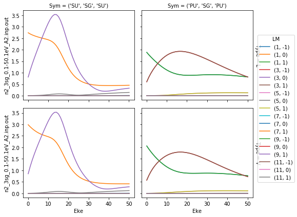
\(N_2\) mutli-E
Calculate \(\beta_{LM}\) as function of energy.
Calculating MFBLMs for 81 pairs... Eke = 0.1 eV, eAngs = ([0, 0, 0])
Calculating MFBLMs for 81 pairs... Eke = 1.1 eV, eAngs = ([0, 0, 0])
Calculating MFBLMs for 81 pairs... Eke = 2.1 eV, eAngs = ([0, 0, 0])
Calculating MFBLMs for 81 pairs... Eke = 3.1 eV, eAngs = ([0, 0, 0])
Calculating MFBLMs for 81 pairs... Eke = 4.1 eV, eAngs = ([0, 0, 0])
Calculating MFBLMs for 81 pairs... Eke = 5.1 eV, eAngs = ([0, 0, 0])
Calculating MFBLMs for 81 pairs... Eke = 6.1 eV, eAngs = ([0, 0, 0])
Calculating MFBLMs for 81 pairs... Eke = 7.1 eV, eAngs = ([0, 0, 0])
Calculating MFBLMs for 81 pairs... Eke = 8.1 eV, eAngs = ([0, 0, 0])
Calculating MFBLMs for 81 pairs... Eke = 9.1 eV, eAngs = ([0, 0, 0])
Calculating MFBLMs for 81 pairs... Eke = 10.1 eV, eAngs = ([0, 0, 0])
Calculating MFBLMs for 81 pairs... Eke = 11.1 eV, eAngs = ([0, 0, 0])
Calculating MFBLMs for 81 pairs... Eke = 12.1 eV, eAngs = ([0, 0, 0])
Calculating MFBLMs for 81 pairs... Eke = 13.1 eV, eAngs = ([0, 0, 0])
Calculating MFBLMs for 81 pairs... Eke = 14.1 eV, eAngs = ([0, 0, 0])
Calculating MFBLMs for 81 pairs... Eke = 15.1 eV, eAngs = ([0, 0, 0])
Calculating MFBLMs for 81 pairs... Eke = 16.1 eV, eAngs = ([0, 0, 0])
Calculating MFBLMs for 81 pairs... Eke = 17.1 eV, eAngs = ([0, 0, 0])
Calculating MFBLMs for 81 pairs... Eke = 18.1 eV, eAngs = ([0, 0, 0])
Calculating MFBLMs for 81 pairs... Eke = 19.1 eV, eAngs = ([0, 0, 0])
Calculating MFBLMs for 81 pairs... Eke = 20.1 eV, eAngs = ([0, 0, 0])
Calculating MFBLMs for 81 pairs... Eke = 21.1 eV, eAngs = ([0, 0, 0])
Calculating MFBLMs for 81 pairs... Eke = 22.1 eV, eAngs = ([0, 0, 0])
Calculating MFBLMs for 81 pairs... Eke = 23.1 eV, eAngs = ([0, 0, 0])
Calculating MFBLMs for 81 pairs... Eke = 24.1 eV, eAngs = ([0, 0, 0])
Calculating MFBLMs for 81 pairs... Eke = 25.1 eV, eAngs = ([0, 0, 0])
Calculating MFBLMs for 81 pairs... Eke = 26.1 eV, eAngs = ([0, 0, 0])
Calculating MFBLMs for 81 pairs... Eke = 27.1 eV, eAngs = ([0, 0, 0])
Calculating MFBLMs for 81 pairs... Eke = 28.1 eV, eAngs = ([0, 0, 0])
Calculating MFBLMs for 81 pairs... Eke = 29.1 eV, eAngs = ([0, 0, 0])
Calculating MFBLMs for 81 pairs... Eke = 30.1 eV, eAngs = ([0, 0, 0])
Calculating MFBLMs for 81 pairs... Eke = 31.1 eV, eAngs = ([0, 0, 0])
Calculating MFBLMs for 81 pairs... Eke = 32.1 eV, eAngs = ([0, 0, 0])
Calculating MFBLMs for 81 pairs... Eke = 33.1 eV, eAngs = ([0, 0, 0])
Calculating MFBLMs for 81 pairs... Eke = 34.1 eV, eAngs = ([0, 0, 0])
Calculating MFBLMs for 81 pairs... Eke = 35.1 eV, eAngs = ([0, 0, 0])
Calculating MFBLMs for 81 pairs... Eke = 36.1 eV, eAngs = ([0, 0, 0])
Calculating MFBLMs for 81 pairs... Eke = 37.1 eV, eAngs = ([0, 0, 0])
Calculating MFBLMs for 81 pairs... Eke = 38.1 eV, eAngs = ([0, 0, 0])
Calculating MFBLMs for 81 pairs... Eke = 39.1 eV, eAngs = ([0, 0, 0])
Calculating MFBLMs for 81 pairs... Eke = 40.1 eV, eAngs = ([0, 0, 0])
Calculating MFBLMs for 81 pairs... Eke = 41.1 eV, eAngs = ([0, 0, 0])
Calculating MFBLMs for 81 pairs... Eke = 42.1 eV, eAngs = ([0, 0, 0])
Calculating MFBLMs for 81 pairs... Eke = 43.1 eV, eAngs = ([0, 0, 0])
Calculating MFBLMs for 81 pairs... Eke = 44.1 eV, eAngs = ([0, 0, 0])
Calculating MFBLMs for 81 pairs... Eke = 45.1 eV, eAngs = ([0, 0, 0])
Calculating MFBLMs for 81 pairs... Eke = 46.1 eV, eAngs = ([0, 0, 0])
Calculating MFBLMs for 81 pairs... Eke = 47.1 eV, eAngs = ([0, 0, 0])
Calculating MFBLMs for 81 pairs... Eke = 48.1 eV, eAngs = ([0, 0, 0])
Calculating MFBLMs for 81 pairs... Eke = 49.1 eV, eAngs = ([0, 0, 0])
Calculating MFBLMs for 81 pairs... Eke = 50.1 eV, eAngs = ([0, 0, 0])
Elapsed time = 42.335490226745605 seconds, for 51 energy points.
<xarray.DataArray (Euler: 1, Eke: 51, BLM: 121)>
array([[[2.301322 +0.j, 0. +0.j, ..., nan+nanj, nan+nanj],
[2.382333 +0.j, 0. +0.j, ..., nan+nanj, nan+nanj],
...,
[0.092948 +0.j, 0. +0.j, ..., 0. +0.j, 0. +0.j],
[0.095428 +0.j, 0. +0.j, ..., 0. +0.j, 0. +0.j]]])
Coordinates:
* Euler (Euler) MultiIndex
- P (Euler) int64 0
- T (Euler) int64 0
- C (Euler) int64 0
* BLM (BLM) MultiIndex
- l (BLM) int64 0 1 1 1 2 2 2 2 2 3 3 ... 10 10 10 10 10 10 10 10 10 10
- m (BLM) int64 0 -1 0 1 -2 -1 0 1 2 -3 -2 ... 0 1 2 3 4 5 6 7 8 9 10
* Eke (Eke) float64 0.1 1.1 2.1 3.1 4.1 5.1 ... 46.1 47.1 48.1 49.1 50.1
Attributes:
Lmax: 11
Targ: SG
QNs: ['m', 'l', 'mu', 'ip', 'it', 'Value']
dataType: BLM
file: n2_3sg_0.1-50.1eV_A2.inp.out
fileBase: D:codegithubePSprocdata
thres: 0.0001
sumDims: ('l', 'm', 'mu', 'Cont', 'Targ', 'Total', 'it')
selDims: [('Type', 'L')]
[<matplotlib.lines.Line2D at 0x1fd4a9a24a8>,
<matplotlib.lines.Line2D at 0x1fd4a9a2fd0>,
<matplotlib.lines.Line2D at 0x1fd4a9a27b8>,
<matplotlib.lines.Line2D at 0x1fd4b84dc18>,
<matplotlib.lines.Line2D at 0x1fd4b84d940>,
<matplotlib.lines.Line2D at 0x1fd4b84d6a0>]

[<matplotlib.lines.Line2D at 0x1fd4adb56a0>,
<matplotlib.lines.Line2D at 0x1fd4adb5710>,
<matplotlib.lines.Line2D at 0x1fd4adb5470>,
<matplotlib.lines.Line2D at 0x1fd4adb5668>,
<matplotlib.lines.Line2D at 0x1fd4adb5358>,
<matplotlib.lines.Line2D at 0x1fd4adb5d30>]

MFPADs: calculate & plot from \(\beta_{LM}\)
Plotting with mpl

[<Figure size 432x288 with 1 Axes>]
N2 test data, MFPADs vs E
<xarray.plot.facetgrid.FacetGrid at 0x1fd4b91f048>

Plotting with mpl
Data dims: ('Euler', 'Eke', 'Theta', 'Phi'), subplots on Eke


[<Figure size 432x288 with 1 Axes>,
<Figure size 432x288 with 1 Axes>,
<Figure size 432x288 with 1 Axes>,
<Figure size 432x288 with 1 Axes>,
<Figure size 432x288 with 1 Axes>]
Plotting with pl
\(NO_2\) (x,y,z) polarizations
Benchmark results, single energy, multiple polarization geometries.
Calculate
Calculating MFBLMs for 12544 pairs... Eke = 0.81 eV, eAngs = ([0. 0. 0.])
Elapsed time = 124.42453789710999 seconds
Calculating MFBLMs for 12544 pairs... Eke = 0.81 eV, eAngs = ([0. 1.57079633 0. ])
Elapsed time = 126.24425601959229 seconds
Calculating MFBLMs for 12544 pairs... Eke = 0.81 eV, eAngs = ([1.57079633 1.57079633 0. ])
Elapsed time = 125.88551211357117 seconds
[<matplotlib.lines.Line2D at 0x1fd627882e8>,
<matplotlib.lines.Line2D at 0x1fd62788e80>,
<matplotlib.lines.Line2D at 0x1fd627889b0>,
<matplotlib.lines.Line2D at 0x1fd62788748>,
<matplotlib.lines.Line2D at 0x1fd62788780>,
<matplotlib.lines.Line2D at 0x1fd62788f60>,
<matplotlib.lines.Line2D at 0x1fd62a4bc50>,
<matplotlib.lines.Line2D at 0x1fd62a4b908>,
<matplotlib.lines.Line2D at 0x1fd62a4b5f8>,
<matplotlib.lines.Line2D at 0x1fd62a4b4a8>,
<matplotlib.lines.Line2D at 0x1fd627e5630>,
<matplotlib.lines.Line2D at 0x1fd62a4b278>,
<matplotlib.lines.Line2D at 0x1fd62a4bb70>,
<matplotlib.lines.Line2D at 0x1fd62a4bba8>,
<matplotlib.lines.Line2D at 0x1fd62a4b828>,
<matplotlib.lines.Line2D at 0x1fd62a16048>,
<matplotlib.lines.Line2D at 0x1fd62a16470>,
<matplotlib.lines.Line2D at 0x1fd62a16128>,
<matplotlib.lines.Line2D at 0x1fd62a167f0>,
<matplotlib.lines.Line2D at 0x1fd62a163c8>,
<matplotlib.lines.Line2D at 0x1fd62a169b0>,
<matplotlib.lines.Line2D at 0x1fd62a16c50>,
<matplotlib.lines.Line2D at 0x1fd62a16eb8>,
<matplotlib.lines.Line2D at 0x1fd62a16c88>,
<matplotlib.lines.Line2D at 0x1fd62a16b70>,
<matplotlib.lines.Line2D at 0x1fd62a170f0>]

MFPADs
Plotting with mpl
Data dims: ('Euler', 'Eke', 'Theta', 'Phi'), subplots on Euler


[<Figure size 432x288 with 1 Axes>,
<Figure size 432x288 with 1 Axes>,
<Figure size 432x288 with 1 Axes>]
Benchmark vs. “direct” results
Compare against results from ep.mfpad, see main “ePSproc demo
notebook”
for calculation details.
MFPADs for test NO2 dataset (single energy, (z,x,y) pol states)
Plotting with mpl

Plotting with mpl

Plotting with mpl

(Visual comparison looks OK, still some benchmarks to to for numerical re/im comparisons, which currently show some differences.)
epsproc package
Submodules
epsproc.IO module
ePSproc IO functions.
Module for file IO and data parsing.
Main function: epsproc.IO.readMatEle():
readMatEle(fileIn = None, fileBase = None, fType = ‘.out’):
Read ePS file(s) and return results as Xarray data structures containing matrix elements. File endings specified by fType, default .out.
History
- 06/11/19 Added jobInfo and molInfo data structures, from ePS file via
epsproc.IO.headerFileParse()andepsproc.IO.molInfoParse(). - Still needs a bit of work, and may want to implement other (comp chem) libraries here.
14/10/19 Added/debugged read functions for CrossSecion segments.
27/09/19 Added read functions for EDCS segments.
- 17/09/19 Added read/write to/from netCDF files for Xarrays.
- Use built-in methods, with work-arounds for complex number format issues.
29/08/19 Updating docs to rst.
- 26/08/19 Added parsing for E, sym parameters from head of ePS file.
- Added error checking by comparing read mat elements to expected list. Changed & fixed Xarray indexing - matrix elements now output with dims (LM, Eke, Sym, mu, it, Type) Current code rather ugly however.
19/08/19 Add functions for reading wavefunction files (3D data)
07/08/19 Naming convention tweaks, and some changes to comments, following basic tests with Sphinx.
- 05/08/19 v1 Initial python version.
- Working, but little error checking as yet. Needs some tidying.
To do
- Add IO for other file segments (only DumpIdy supported so far).
- Better logic & flexibility for file scanning.
- Restructure as class for brevity…?
- More sophisticated methods/data structures for job & molecule info handling.
-
epsproc.IO.EDCSFileParse(fileName)[source]¶ Parse an ePS file for EDCS segments.
Parameters: fileName (str) – File to read (file in working dir, or full path) Returns: - list – [lineStart, lineStop], ints for line #s found from start and end phrases.
- list – dumpSegs, list of lines read from file.
- Lists contain entries for each dumpIdy segment found in the file.
-
epsproc.IO.EDCSSegParse(dumpSeg)[source]¶ Extract values from EDCS file segments.
Parameters: dumpSeg (list) – One EDCS segment, from dumpSegs[], as returned by epsproc.IO.EDCSFileParse()Returns: - np.array – EDCS, array of scattering XS, [theta, Cross Section (Angstrom^2)]
- list – attribs, list [Label, value, units]
Notes
Currently this is a bit messy, and relies on fixed EDCS format. No error checking as yet. Not yet reading all attribs.
Example
>>> EDCS, attribs = EDCSSegParse(dumpSegs[0])
-
epsproc.IO.EDCSSegsParseX(dumpSegs)[source]¶ Extract data from ePS EDCS segments into usable form.
Parameters: dumpSegs (list) – Set of dumpIdy segments, i.e. dumpSegs, as returned by epsproc.IO.EDCSFileParse()Returns: - xr.array – Xarray data array, containing cross sections. Dimensions (Eke, theta)
- int – Number of blank segments found. (CURRENTLY not implemented.)
Example
>>> data = EDCSSegsParseX(dumpSegs)
Notes
A rather cut-down version of
epsproc.IO.dumpIdySegsParseX(), no error checking currently implemented.
-
epsproc.IO.dumpIdyFileParse(fileName)[source]¶ Parse an ePS file for dumpIdy segments.
Parameters: fileName (str) – File to read (file in working dir, or full path) Returns: - list – [lineStart, lineStop], ints for line #s found from start and end phrases.
- list – dumpSegs, list of lines read from file.
- Lists contain entries for each dumpIdy segment found in the file.
-
epsproc.IO.dumpIdySegParse(dumpSeg)[source]¶ Extract values from dumpIdy file segments.
Parameters: dumpSeg (list) – One dumpIdy segment, from dumpSegs[], as returned by epsproc.IO.dumpIdyFileParse()Returns: - np.array – rawIdy, array of matrix elements, [m,l,mu,ip,it,Re,Im]
- list – attribs, list [Label, value, units]
Notes
Currently this is a bit messy, and relies on fixed DumpIDY format. No error checking as yet. Not yet reading all attribs.
Example
>>> matEle, attribs = dumpIdySegParse(dumpSegs[0])
-
epsproc.IO.dumpIdySegsParseX(dumpSegs, ekeListUn, symSegs)[source]¶ Extract data from ePS dumpIdy segments into usable form.
Parameters: - dumpSegs (list) – Set of dumpIdy segments, i.e. dumpSegs, as returned by
epsproc.IO.dumpIdyFileParse() - ekeListUn (list) – List of energies, used for error-checking and Xarray rearraging, as returned by
epsproc.IO.scatEngFileParse()
Returns: - xr.array – Xarray data array, containing matrix elements etc. Dimensions (LM, Eke, Sym, mu, it, Type)
- int – Number of blank segments found.
Example
>>> data = dumpIdySegsParseX(dumpSegs)
- dumpSegs (list) – Set of dumpIdy segments, i.e. dumpSegs, as returned by
-
epsproc.IO.fileParse(fileName, startPhrase=None, endPhrase=None, comment=None, verbose=False)[source]¶ Parse a file, return segment(s) from startPhrase:endPhase, excluding comments.
Parameters: - fileName (str) – File to read (file in working dir, or full path)
- startPhrase (str, optional) – Phrase denoting start of section to read. Default = None
- endPhase (str, optional) – Phrase denoting end of section to read. Default = None
- comment (str, optional) – Phrase denoting comment lines, which are skipped. Default = None
Returns: - list – [lineStart, lineStop], ints for line #s found from start and end phrases.
- list – segments, list of lines read from file.
- All lists can contain multiple entries, if more than one segment matches the search criteria.
-
epsproc.IO.getCroFileParse(fileName)[source]¶ Parse an ePS file for GetCro/CrossSection segments.
Parameters: fileName (str) – File to read (file in working dir, or full path) Returns: - list – [lineStart, lineStop], ints for line #s found from start and end phrases.
- list – dumpSegs, list of lines read from file.
- Lists contain entries for each dumpIdy segment found in the file.
-
epsproc.IO.getCroSegParse(dumpSeg)[source]¶ Extract values from GetCro/CrossSection file segments.
Parameters: dumpSeg (list) – One CrossSection segment, from dumpSegs[], as returned by epsproc.IO.getCroFileParse()Returns: - np.array – CrossSections, table of results vs. energy.
- list – attribs, list [Label, value, units]
Notes
Currently this is a bit messy, and relies on fixed CrossSection output format. No error checking as yet. Not yet reading all attribs.
Example
>>> XS, attribs = getCroSegParse(dumpSegs[0])
-
epsproc.IO.getCroSegsParseX(dumpSegs, symSegs, ekeList)[source]¶ Extract data from ePS getCro/CrossSecion segments into usable form.
Parameters: dumpSegs (list) – Set of dumpIdy segments, i.e. dumpSegs, as returned by epsproc.IO.getCroFileParse()Returns: - xr.array – Xarray data array, containing cross sections. Dimensions (Eke, theta)
- int – Number of blank segments found. (CURRENTLY not implemented.)
Example
>>> data = getCroSegsParseX(dumpSegs)
Notes
A rather cut-down version of
epsproc.IO.dumpIdySegsParseX(), no error checking currently implemented.
-
epsproc.IO.getFiles(fileIn=None, fileBase=None, fType='.out')[source]¶ Read ePS file(s) and return results as Xarray data structures. File endings specified by fType, default .out.
Parameters: - fileIn (str, list of strs, optional.) – File(s) to read (file in working dir, or full path).
Defaults to current working dir if only a file name is supplied.
For consistent results, pass raw strings, e.g.
fileIn = r"C:\share\code\ePSproc\python_dev\no2_demo_ePS.out" - fileBase (str, optional.) – Dir to scan for files. Currently only accepts a single dir. Defaults to current working dir if no other parameters are passed.
- fType (str, optional) – File ending for ePS output files, default ‘.out’
Returns: List of Xarray data arrays, containing matrix elements etc. from each file scanned.
Return type: list
- fileIn (str, list of strs, optional.) – File(s) to read (file in working dir, or full path).
Defaults to current working dir if only a file name is supplied.
For consistent results, pass raw strings, e.g.
-
epsproc.IO.headerFileParse(fileName, verbose=True)[source]¶ Parse an ePS file for header & input job info.
Parameters: - fileName (str) – File to read (file in working dir, or full path)
- verbose (bool, default True) – Print job info from file header if true.
Returns: - jobInfo (dict) – Dictionary generated from job details.
- TO DO
- —–
- - Tidy up methods - maybe with parseDigits?
- - Tidy up dict output.
-
epsproc.IO.matEleGroupDim(data, dimGroups=[3, 4, 2])[source]¶ Group ePS matrix elements by redundant labels.
Default is to group by [‘ip’, ‘it’, ‘mu’] terms, all have only a few values.
TODO: better ways to do this? Shoud be possible at Xarray level.
Parameters: data (list) – Sections from dumpIdy segment, as created in dumpIdySegsParseX() Ordering is [labels, matElements, attribs].
-
epsproc.IO.matEleGroupDimX(daIn)[source]¶ Group ePS matrix elements by redundant labels (Xarray version).
Group by [‘ip’, ‘it’, ‘mu’] terms, all have only a few values. Rename ‘ip’:1,2 as ‘Type’:’L’,’V’
TODO: better ways to do this? Via Stack/Unstack? http://xarray.pydata.org/en/stable/api.html#id16 See also tests in funcTests_210819.py for more versions/tests.
Parameters: data (Xarray) – Data array with matrix elements to be split and recombined by dims. Returns: data – Data array with reordered matrix elements (dimensions). Return type: Xarray
-
epsproc.IO.matEleGroupDimXnested(da)[source]¶ Group ePS matrix elements by redundant labels (Xarray version).
Group by [‘ip’, ‘it’, ‘mu’] terms, all have only a few values.
TODO: better ways to do this? See also tests in funcTests_210819.py for more versions/tests.
Parameters: data (Xarray) – Data array with matrix elements to be split and recombined by dims.
-
epsproc.IO.molInfoParse(fileName, verbose=True)[source]¶ Parse an ePS file for header & input job info.
Parameters: - fileName (str) – File to read (file in working dir, or full path)
- verbose (bool, default True) – Print job info from file header if true.
Returns: molInfo – Dictionary with atom & orbital details.
Return type: dict
-
epsproc.IO.parseLineDigits(testLine)[source]¶ Use regular expressions to extract digits from a string. https://stackoverflow.com/questions/4289331/how-to-extract-numbers-from-a-string-in-python
-
epsproc.IO.readMatEle(fileIn=None, fileBase=None, fType='.out', recordType='DumpIdy')[source]¶ Read ePS file(s) and return results as Xarray data structures. File endings specified by fType, default *.out.
Parameters: - fileIn (str, list of strs, optional.) – File(s) to read (file in working dir, or full path).
Defaults to current working dir if only a file name is supplied.
For consistent results, pass raw strings, e.g.
fileIn = r"C:\share\code\ePSproc\python_dev\no2_demo_ePS.out" - fileBase (str, optional.) – Dir to scan for files. Currently only accepts a single dir. Defaults to current working dir if no other parameters are passed.
- fType (str, optional) – File ending for ePS output files, default ‘.out’
- recordType (str, optional, default 'DumpIdy') – Type of record to scan for, currently set for ‘DumpIdy’, ‘EDCS’ or ‘CrossSection’. For a full list of descriptions, types and sources, run: >>> epsproc.util.dataTypesList()
Returns: List of Xarray data arrays, containing matrix elements etc. from each file scanned.
Return type: list
Examples
>>> dataSet = readMatEle() # Scan current dir
>>> fileIn = r'C:\share\code\ePSproc\python_dev\no2_demo_ePS.out' >>> dataSet = readMatEle(fileIn) # Scan single file
>>> dataSet = readMatEle(fileBase = r'C:\share\code\ePSproc\python_dev') # Scan dir
Note
- Files are scanned for matrix element output flagged by “DumpIdy” headers.
- Each segment found is parsed for attributes and data (set of matrix elements).
- Matrix elements and attributes are combined and output as an Xarray array.
- fileIn (str, list of strs, optional.) – File(s) to read (file in working dir, or full path).
Defaults to current working dir if only a file name is supplied.
For consistent results, pass raw strings, e.g.
-
epsproc.IO.readOrb3D(fileIn=None, fileBase=None, fType='_Orb.dat')[source]¶ Read ePS 3D data file(s) and return results. File endings specified by fType, default *_Orb.dat.
- fileIn : str, list of strs, optional.
- File(s) to read (file in working dir, or full path). Defaults to current working dir if only a file name is supplied. For consistent results, pass raw strings, e.g. fileIn = r”C:sharecodeePSprocpython_dev
o2_demo_ePS.out”
- fileBase : str, optional.
- Dir to scan for files. Currently only accepts a single dir. Defaults to current working dir if no other parameters are passed.
- fType : str, optional
- File ending for ePS output files, default ‘_Orb.dat’
- list
- List of data arrays, containing matrix elements etc. from each file scanned.
# TODO: Change output to Xarray?
>>> dataSet = readOrb3D() # Scan current dir
>>> fileIn = r'C:\share\code\ePSproc\python_dev\DABCOSA2PPCA2PP_10.5eV_Orb.dat' >>> dataSet = readOrb3D(fileIn) # Scan single file
>>> dataSet = readOrb3D(fileBase = r'C:\share\code\ePSproc\python_dev') # Scan dir
-
epsproc.IO.readXarray(fileName, filePath=None)[source]¶ Read file from netCDF format via Xarray method.
Parameters: - fileName (str) – File to read.
- filePath (str, optional, default = None) – Full path to file. If set to None (default) the file will be written in the current working directory (as returned by os.getcwd()).
Returns: Data from file. May be in serialized format.
Return type: Xarray
Notes
The default option for Xarray is to use Scipy netCDF writer, which does not support complex datatypes. In this case, the data array is written as a dataset with a real and imag component.
Multi-level indexing is also not supported, and must be serialized first. Ugh.
TODO: generalize multi-level indexing here.
-
epsproc.IO.scatEngFileParse(fileName)[source]¶ Parse an ePS file for ScatEng list.
Parameters: fileName (str) – File to read (file in working dir, or full path) Returns: - list – ekeList, np array of energies set in the ePS file.
- Lists contain entries for each dumpIdy segment found in the file.
-
epsproc.IO.symFileParse(fileName)[source]¶ Parse an ePS file for ScatEng list.
Parameters: fileName (str) – File to read (file in working dir, or full path) Returns: - list – symSegs, raw lines from the ePS file.
- Lists contain entries for each dumpIdy segment found in the file.
-
epsproc.IO.writeOrb3Dvtk(dataSet)[source]¶ Write ePS 3D data file(s) to vtk format. This can be opened in, e.g., Paraview.
Parameters: - dataSet (list) – List of data arrays, containing matrix elements etc. from each file scanned. Assumes format as output by readOrb3D(), [fileName, headerLines, coords, data]
- TODO (#) –
Returns: List of output files.
Return type: list
-
epsproc.IO.writeXarray(dataIn, fileName=None, filePath=None)[source]¶ Write file to netCDF format via Xarray method.
Parameters: - dataIn (Xarray) – Data array to write to disk.
- fileName (str, optional, default = None) – Filename to use. If set to None (default) the file will be written with a datastamp.
- filePath (str, optional, default = None) – Full path to file. If set to None (default) the file will be written in the current working directory (as returned by os.getcwd()).
Returns: Indicates save type and file path.
Return type: str
Notes
The default option for Xarray is to use Scipy netCDF writer, which does not support complex datatypes. In this case, the data array is written as a dataset with a real and imag component.
TODO: implement try/except to handle various cases here, and test other netCDF writers (see http://xarray.pydata.org/en/stable/io.html#netcdf).
Multi-level indexing is also not supported, and must be serialized first. Ugh.
epsproc.MFBLM module
ePSproc MFBLM functions
23/09/19 Testing function caching…
19/09/19 Working & verified basic version (slow loop).
- 05/09/19 v1 Initial python version.
- Based on original Matlab code ePS_MFBLM.m
Formalism
Should be something like this, with possible substitutions or phase swaps.
Exact numerics may vary.
-
epsproc.MFBLM.MFBLMCalcLoop(matE, eAngs=[0, 0, 0], thres=1e-06, p=0, R=0, verbose=1)[source]¶ Calculate inner loop for MFBLMs, based on passed set of matrix elements (Xarray).
Loop code based on Matlab code ePSproc_MFBLM.m
This works, but not very clean or efficient - should be possible to parallelize & vectorise… but this is OK for testing, benchmarking and verification purposes.
Parameters: - matE (Xarray) – Contains one set of matrix elements to use for calculation. Currently assumes these are a 1D list, with associated (l,m,mu) parameters, as set by mfblm().
- eAngs ([phi,theta,chi], optional, default = [0,0,0]) – Single set of Euler angles defining polarization geometry.
- thres (float, optional, default = 1e-4) – Threshold value for testing significance of terms. Terms < thres will be dropped.
- p (int, optional, default p = 0) – LF polarization term. Currently only valid for p = 0
- R (int, optional, default R = 0) – LF polarization term (from tensor contraction). Currently only valid for p = 0
- verbose (int, optional, default 1) –
Verbosity level:
- 0: Silent run.
- 1: Print basic info.
- 2: Print intermediate C parameter array to termina when running.
Returns: - BLMX (Xarray) – Set of B(L,M; eAngs, Eke) terms for supplied matrix elements, in an Xarray. For cases where no values are calculated (below threshold), return an array with B00 = 0 only.
- Limitations & To Do
- ——————–
- * Currently set with (p,R) values passed, but only valid for (0,0) (not full sum over R terms as shown in formalism above.)
- * Set to accept a single set of matrix elements (single E), assuming looping over E (and other parameters) elsewhere.
- * Not explicitly parallelized here, should be done by calling function.
- (Either via Xarray methods, or numba/dask…? http (//xarray.pydata.org/en/stable/computation.html#wrapping-custom-computation))
- * Coded for ease, not efficiency - there will be lots of repeated ang. mom. calcs. when run over many sets of matrix elements.
- * Scale factor currently not propagated.
-
epsproc.MFBLM.blmXarray(BLM, Eke)[source]¶ Create Xarray from BLM list, format BLM = [L, M, Beta], at a single energy Eke.
Array sorting only valid for 2D BLM array, for B00=0 case pass BLM = None.
-
epsproc.MFBLM.mfblm(da, selDims={'Type': 'L'}, eAngs=[0, 0, 0], thres=0.0001, sumDims=('l', 'm', 'mu', 'Cont', 'Targ', 'Total', 'it'), SFflag=True, verbose=1)[source]¶ Calculate MFBLMs for a range of (E, sym) cases. Default is to calculated for all symmetries at each energy.
Parameters: - da (Xarray) – Contains matrix elements to use for calculation. Matrix elements will be sorted by energy and BLMs calculated for each set.
- selDims (dict, optional, default = {'Type':'L'}) – Additional sub-selection to be applied to matrix elements before BLM calculation. Default selects just length gauge results.
- eAngs ([phi,theta,chi], optional, default = [0,0,0]) – Single set of Euler angles defining polarization geometry.
- thres (float, optional, default = 1e-4) – Threshold value for testing significance of terms. Terms < thres will be dropped.
- sumDims (tuple, optional, default = ('l','m','mu','Cont','Targ','Total','it')) – Defines which terms are summed over (coherent) in the MFBLM calculation. (These are used to flatten the Xarray before calculation.) Default includes sum over (l,m), symmetries and degeneracies (but not energies).
- SFflag (bool, default = True) – Normalise by scale factor to give X-sections (B00) in Mb
- verbose (int, optional, default 1) –
Verbosity level:
- 0: Silent run.
- 1: Print basic info.
- 2: Print intermediate C parameter array to termina when running.
Returns: - Xarray – Calculation results BLM, dims (Euler, Eke, l,m). Some global attributes are also appended.
- Limitations
- ———–
- Currently set to loop calcualtions over energy only, and all symmetries.
- Pass single {‘Cont’ (‘sym’} to calculated for only one symmetry group.)
- TODO (In future this will be more elegant.)
- TODO (Setting selDims in output structure needs more thought for netCDF save compatibility.)
-
epsproc.MFBLM.mfblmEuler(da, selDims={'Type': 'L'}, eAngs=[0, 0, 0], thres=0.0001, sumDims=('l', 'm', 'mu', 'Cont', 'Targ', 'Total', 'it'), SFflag=True, verbose=1)[source]¶ Wrapper for epsproc.mfblm() for a set of Euler angles. All other parameters are simply passed to mfblm(). Calculate MFBLMs for a range of (E, sym) cases. Default is to calculated for all symmetries at each energy.
Parameters: - da (Xarray) – Contains matrix elements to use for calculation. Matrix elements will be sorted by energy and BLMs calculated for each set.
- selDims (dict, optional, default = {'Type':'L'}) – Additional sub-selection to be applied to matrix elements before BLM calculation. Default selects just length gauge results.
- eAngs ([phi,theta,chi], optional, default = [0,0,0]) – Set of Euler angles defining polarization geometry. List or np.array, dims(N, 3).
- thres (float, optional, default = 1e-4) – Threshold value for testing significance of terms. Terms < thres will be dropped.
- sumDims (tuple, optional, default = ('l','m','mu','Cont','Targ','Total','it')) – Defines which terms are summed over (coherent) in the MFBLM calculation. (These are used to flatten the Xarray before calculation.) Default includes sum over (l,m), symmetries and degeneracies (but not energies).
- SFflag (bool, default = True) – Normalise by scale factor to give X-sections (B00) in Mb
- verbose (int, optional, default 1) –
Verbosity level:
- 0: Silent run.
- 1: Print basic info.
- 2: Print intermediate C parameter array to termina when running.
Returns: - Xarray – Calculation results BLM, dims (Euler, Eke, l,m). Some global attributes are also appended.
- Limitations
- ———–
- Currently set to loop calcualtions over energy only, and all symmetries.
- Pass single {‘Cont’ (‘sym’} to calculated for only one symmetry group.)
- TODO (In future this will be more elegant.)
- TODO (Setting selDims in output structure needs more thought for netCDF save compatibility.)
epsproc.MFPAD module
ePSproc MFPAD functions
- 05/08/19 v1 Initial python version.
- Based on original Matlab code ePS_MFPAD.m
Structure
Calculate MFPAD on a grid from input ePS matrix elements. Use fast functions, pre-calculate if possible. Data in Xarray, use selection functions and multiplications based on relevant quantum numbers, other axes summed over.
- Choices for functions…
Moble’s spherical functions (quaternion based)
Provides fast wignerD, 3j and Ylm functions, uses Numba.
Install with:
>>> conda install -c conda-forge spherical_functions
To Do
- Propagate scale-factor to Mb.
- Benchmark on NO2 reference results.
- ~~Test over multiple E.~~
- Test over multiple R.
- More efficient computation? Use Xarray group by?
Formalism
From ePSproc: Post-processing suite for ePolyScat electron-molecule scattering calculations.
In this formalism:
- \(I_{l,m,\mu}^{p_{i}\mu_{i},p_{f}\mu_{f}}(E)\) is the radial part of the dipole matrix element, determined from the initial and final state electronic wavefunctions \(\Psi_{i}^{p_{i},\mu_{i}}\) and \(\Psi_{f}^{p_{f},\mu_{f}}\), photoelectron wavefunction \(\varphi_{klm}^{(-)}\) and dipole operator \(\hat{d_{\mu}}\). Here the wavefunctions are indexed by irreducible representation (i.e. symmetry) by the labels \(p_{i}\) and \(p_{f}\), with components \(\mu_{i}\) and \(\mu_{f}\) respectively; \(l,m\) are angular momentum components, \(\mu\) is the projection of the polarization into the MF (from a value \(\mu_{0}\) in the LF). Each energy and irreducible representation corresponds to a calculation in ePolyScat.
- \(T_{\mu_{0}}^{p_{i}\mu_{i},p_{f}\mu_{f}}(\theta_{\hat{k}},\phi_{\hat{k}},\theta_{\hat{n}},\phi_{\hat{n}})\) is the full matrix element (expanded in polar coordinates) in the MF, where \(\hat{k}\) denotes the direction of the photoelectron \(\mathbf{k}\)-vector, and \(\hat{n}\) the direction of the polarization vector \(\mathbf{n}\) of the ionizing light. Note that the summation over components \(\{l,m,\mu\}\) is coherent, and hence phase sensitive.
- \(Y_{lm}^{*}(\theta_{\hat{k}},\phi_{\hat{k}})\) is a spherical harmonic.
- \(D_{\mu,\mu_{0}}^{1}(R_{\hat{n}})\) is a Wigner rotation matrix element, with a set of Euler angles \(R_{\hat{n}}=(\phi_{\hat{n}},\theta_{\hat{n}},\chi_{\hat{n}})\), which rotates/projects the polarization into the MF.
- \(I_{\mu_{0}}(\theta_{\hat{k}},\phi_{\hat{k}},\theta_{\hat{n}},\phi_{\hat{n}})\) is the final (observable) MFPAD, for a polarization \(\mu_{0}\) and summed over all symmetry components of the initial and final states, \(\mu_{i}\) and \(\mu_{f}\). Note that this sum can be expressed as an incoherent summation, since these components are (by definition) orthogonal.
- \(g_{p_{i}}\) is the degeneracy of the state \(p_{i}\).
-
epsproc.MFPAD.mfpad(dataIn, thres=0.01, inds={'Type': 'L', 'it': 1}, res=50, R=None, p=0)[source]¶ Parameters: - dataIn (Xarray) – Contains set(s) of matrix elements to use, as output by epsproc.readMatEle().
- thres (float, optional, default 1e-2) – Threshold value for matrix elements to use in calculation.
- ind (dictionary, optional.) – Used for sub-selection of matrix elements from Xarrays. Default set for length gauage, single it component only, inds = {‘Type’:’L’,’it’:‘1’}.
- res (int, optional, default 50) – Resolution for output (theta,phi) grids.
- R (list of Euler angles or quaternions, optional.) – Define LF > MF polarization geometry/rotations. For default case (R = None), 3 geometries are calculated, corresponding to z-pol, x-pol and y-pol cases. Defined by Euler angles (p,t,c) = [0 0 0] for z-pol, [0 pi/2 0] for x-pol, [pi/2 pi/2 0] for y-pol.
- p (int, optional.) – Defines LF polarization state, p = -1…1, default p = 0 (linearly pol light along z-axis). TODO: add summation over p for multiple pol states in LF.
Returns: - Ta – Xarray (theta, phi, E, Sym) of MFPADs, summed over (l,m)
- Tlm – Xarray (theta, phi, E, Sym, lm) of MFPAD components, expanded over all (l,m)
epsproc.basicPlotters module
ePSproc basic plotting functions
Some basic functions for 2D/3D plots.
07/11/19 v1
-
class
epsproc.basicPlotters.Arrow3D(xs, ys, zs, *args, **kwargs)[source]¶ Bases:
matplotlib.patches.FancyArrowPatchDefine Arrow3D plotting class
Code verbatim from StackOverflow post https://stackoverflow.com/a/22867877 Thanks to CT Zhu, https://stackoverflow.com/users/2487184/ct-zhu
epsproc.sphCalc module
ePSproc spherical function calculations.
Collection of functions for calculating Ylm, wignerD etc.
For spherical harmonics, currently using scipy.special.sph_harm
For other functions, using Moble’s spherical_functions package https://github.com/moble/spherical_functions
See tests/Spherical function testing Aug 2019.ipynb
27/08/19 Added wDcalc for Wigner D functions. 14/08/19 v1 Implmented sphCalc
-
epsproc.sphCalc.sphCalc(Lmax, Lmin=0, res=None, angs=None, XFlag=True)[source]¶ Calculate set of spherical harmonics Ylm(theta,phi) on a grid.
Parameters: - Lmax (int) – Maximum L for the set. Ylm calculated for Lmin:Lmax, all m.
- Lmin (int, optional, default 0) – Min L for the set. Ylm calculated for Lmin:Lmax, all m.
- res (int, optional, default None) – (Theta, Phi) grid resolution, outputs will be of dim [res,res].
- angs (list of 2D np.arrays, [thetea, phi], optional, default None) – If passed, use these grids for calculation
- XFlag (bool, optional, default True) – Flag for output. If true, output is Xarray. If false, np.arrays
- that either res OR angs needs to be passed. (Note) –
- Outputs –
- ------- –
- if XFlag - (-) –
- YlmX – 3D Xarray, dims (lm,theta,phi)
- else - (-) –
- lm (Ylm,) – 3D np.array of values, dims (lm,theta,phi), plus list of lm pairs
-
Currently set for scipy.special.sph_harm as calculation routine.
Example
>>> YlmX = sphCalc(2, res = 50)
-
epsproc.sphCalc.wDcalc(Lrange=[0, 1], Nangs=None, eAngs=None, R=None, XFlag=True)[source]¶ Calculate set of Wigner D functions D(l,m,mp,R) on a grid.
Parameters: - Lrange (list, optional, default [0, 1]) – Range of L to calculate parameters for. If len(Lrange) == 2 assumed to be of form [Lmin, Lmax], otherwise list is used directly. For a given l, all (m, mp) combinations are calculated.
- for setting angles (use one only) (Options) –
- Nangs (int, optional, default None) – If passed, use this to define Euler angles sampled. Ranges will be set as (theta, phi, chi) = (0:pi, 0:pi/2, 0:pi) in Nangs steps.
- eAngs (np.array, optional, default None) – If passed, use this to define Euler angles sampled. Array of angles, [theta,phi,chi], in radians
- R (np.array, optional, default None) – If passed, use this to define Euler angles sampled. Array of quaternions, as given by quaternion.from_euler_angles(eAngs).
- XFlag : bool, optional, default True
- Flag for output. If true, output is Xarray. If false, np.arrays
- if XFlag -
- wDX
- Xarray, dims (lmmp,Euler)
- else -
- wD, R, lmmp
- np.arrays of values, dims (lmmp,Euler), plus list of angles and lmmp sets.
-
Uses Moble's spherical_functions package for wigner D function.
-
https://github.com/moble/spherical_functions
-
Moble's quaternion package for angles and conversions.
-
https://github.com/moble/quaternion
Examples
>>> wDX1 = wDcalc(eAngs = np.array([0,0,0]))
>>> wDX2 = wDcalc(Nangs = 10)
epsproc.sphPlot module
ePSproc spherical polar plotting functions
Collection of functions for plotting 2D spherical polar data \(I(\theta, \phi)\).
Main plotters are:
sphSumPlotX()for arrays of \(I(\theta,\phi)\)sphFromBLMPlot()for arrays of \(\beta_{LM}\) parameters.
13/09/19
- Added sphFromBLMPlot().
- Some additional plot type fuctionality added.
- Some tidying up and reorganising… hopefully nothing broken…
14/08/19 v1
-
epsproc.sphPlot.plotTypeSelector(dataPlot, pType='a')[source]¶ Set plotting data type.
Parameters: - dataPlot (np.array, Xarray) – Data for plotting, output converted to type defined by pType.
- pType (char, optional, default 'a') –
Set type of plot.
- ’a’ (abs) = np.abs(dataPlot)
- ’r’ (real) = np.real(dataPlot)
- ’i’ (imag) = np.imag(dataPlot)
- ’p’ (product) = dataPlot * np.conj(dataPlot)
Returns: Input data structure converted to pType.
Return type: Xarray, np.array
-
epsproc.sphPlot.sphFromBLMPlot(BLMXin, res=50, pType='r', plotFlag=False, facetDim=None, backend='mpl')[source]¶ Calculate spherical harmonic expansions from BLM parameters and plot.
Surfaces calculated as:
\[I(\theta,\phi)=\sum_{L,M}\beta_{L,M}Y_{L,M}(\theta,\phi)\]Parameters: - dataIn (Xarray) – Input set of BLM parameters.
- res (int, optional, default 50) – Resolution for output (theta,phi) grids.
- pType (char, optional, default 'r' (real part)) – Set (data) type to plot. See
plotTypeSelector(). - plotFlag (bool, optional, default False) – Set plotting True/False. Note that this will plot for all facetDim.
- facetDim (str, optional, default None) – Dimension to use for subplots. Currently set for a single dimension only. For matplotlib backend: one figure per surface. For plotly backend: subplots per surface.
- backend (str, optional, default 'mpl' (matplotlib)) – Set backend used for plotting. See
sphSumPlotX()for details.
Returns: - Xarray – Xarray containing the calcualted surfaces I(theta,phi,…)
- fig – List of figure handles.
-
epsproc.sphPlot.sphPlotMPL(dataPlot, theta, phi)[source]¶ Plot spherical polar function (R,theta,phi) to a Cartesian grid, using Matplotlib.
Parameters: - dataPlot (np.array or Xarray) – Values to plot, single surface only, with dims (theta,phi).
- phi (theta,) – Angles defining spherical polar grid, 2D arrays.
Returns: Handle to matplotlib figure.
Return type: fig
-
epsproc.sphPlot.sphPlotPL(dataPlot, theta, phi, facetDim='Eke', rc=None)[source]¶ Plot spherical polar function (R,theta,phi) to a Cartesian grid, using Plotly.
Parameters: - dataPlot (np.array or Xarray) – Values to plot, single surface only, with dims (theta,phi).
- phi (theta,) – Angles defining spherical polar grid, 2D arrays.
- facetDim (str, default 'Eke') – Dimension to use for faceting (subplots), currently set for single dim only.
Returns: Handle to figure.
Return type: fig
-
epsproc.sphPlot.sphSumPlotX(dataIn, pType='a', facetDim='Eke', backend='mpl')[source]¶ Plot sum of spherical harmonics from an Xarray.
Parameters: - dataIn (Xarray) –
Input structure can be
- Set of precalculated Ylms, dims (theta,phi) or (theta,phi,LM).
- Set of precalculated mfpads, dims (theta,phi), (theta,phi,LM) or (theta,phi,LM,facetDim).
- If (LM) dimension is present, it is summed over before plotting.
- If facetDim is present this is used for subplots, currently only one facetDim is supported here.
- pType (char, optional, default 'a' (abs value)) – Set (data) type of plot. See
plotTypeSelector(). - facetDim (str, optional, default Eke) –
Dimension to use for subplots.
- Currently set for a single dimension only.
- For matplotlib backend: one figure per surface.
- For plotly backend: subplots per surface.
- backend (str, optional, default 'mpl') –
Set backend used for plotting.
- mpl matplotlib: basic 3D plotting, one figure per surface.
- pl plotly: fancier 3D plotting, interactive in Jupyter but may fail at console.
- Subplots for surfaces.
- hv holoviews: fancier plotting with additional back-end options.
- Can facet on specific data types.
Returns: List of figure handles.
Return type: fig
Examples
>>> YlmX = sphCalc(2, res = 50) >>> sphSumPlotX(YlmX)
Note
Pretty basic functionality here, should add more colour mapping options and multiple plots, alternative back-ends, support for more dimensions etc.
- dataIn (Xarray) –
-
epsproc.sphPlot.sphToCart(R, theta, phi)[source]¶ Convert spherical polar coords \((R,\theta,\phi)\) to Cartesian \((X,Y,Z)\).
Parameters: theta, phi (R,) – Spherical polar coords \((R,\theta,\phi)\). Returns: X, Y, Z – Cartesian coords \((X,Y,Z)\). Return type: np.arrays Conversion defined with the usual physics convention , where:
- \(R\) is the radial distance from the origin
- \(\theta\) is the polar angle (defined relative to the z-axis), \(0\leq\theta\leq\pi\)
- \(\phi\) is the azimuthal angle (defined relative to the x-axis), \(0\leq\theta\leq2\pi\)
- \(X = R * np.sin(phi) * np.cos(theta)\)
- \(Y = R * np.sin(phi) * np.sin(theta)\)
- \(Z = R * np.cos(phi)\)
epsproc.util module
ePSproc utility functions
Collection of small functions for sorting etc.
14/10/19 Added string replacement function (generic) 11/08/19 Added matEleSelector
-
epsproc.util.BLMdimList(sType='stacked')[source]¶ Return standard list of dimensions for calculated BLM.
Parameters: sType (string, optional, default = 'stacked') – Selected ‘stacked’ or ‘unstacked’ dimensions. Set ‘sDict’ to return a dictionary of unstacked <> stacked dims mappings for use with xr.stack({dim mapping}). Returns: list Return type: set of dimension labels.
-
epsproc.util.dataTypesList()[source]¶ Return a dict of allowed dataTypes, corresponding to epsproc processed data.
Each dataType lists ‘source’, ‘desc’ and ‘recordType’ fields.
- ‘source’ fields correspond to ePS functions which get or generate the data.
- ‘desc’ brief description of the dataType.
- ‘recordType’ gives the required segment in ePS files (and associated parser). If the segment is not present in the source file, then the dataType will not be available.
TODO: best choice of data structure here? Currently nested dictionary.
-
epsproc.util.jobSummary(jobInfo=None, molInfo=None)[source]¶ Print some jobInfo stuff & plot molecular structure. (Currently very basic.)
Parameters: - jobInfo (dict, default = None) – Dictionary of job data, as generated by :py:function:`epsproc.IO.headerFileParse()` from source ePS output file.
- molInfo (dict, default = None) – Dictionary of molecule data, as generated by
epsproc.IO.molInfoParse()from source ePS output file.
-
epsproc.util.matEdimList(sType='stacked')[source]¶ Return standard list of dimensions for matrix elements.
Parameters: sType (string, optional, default = 'stacked') – Selected ‘stacked’ or ‘unstacked’ dimensions. Set ‘sDict’ to return a dictionary of unstacked <> stacked dims mappings for use with xr.stack({dim mapping}). Returns: list Return type: set of dimension labels.
-
epsproc.util.matEleSelector(da, thres=None, inds=None, dims=None, sq=False, drop=True)[source]¶ Select & threshold raw matrix elements in an Xarray
Parameters: - da (Xarray) – Set of matrix elements to sub-select
- thres (float, optional, default None) – Threshold value for abs(matElement), keep only elements > thres. This is element-wise.
- inds (dict, optional, default None) – Dicitonary of additional selection criteria, in name:value format. These correspond to parameter dimensions in the Xarray structure. E.g. inds = {‘Type’:’L’,’Cont’:’A2’}
- dims (str or list of strs, dimensions to look for max & threshold, default None) – Set for dimension-wise thresholding. If set, this is used instead of element-wise thresholding. List of dimensions, which will be checked vs. threshold for max value, according to abs(dim.max) > threshold This allows for consistent selection of continuous parameters over a dimension, by a threshold.
- sq (bool, optional, default False) – Squeeze output singleton dimensions.
- drop (bool, optional, default True) – Passed to da.where() for thresholding, drop coord labels for values below threshold.
Returns: Xarray structure of selected matrix elements. Note that Nans are dropped if possible.
Return type: daOut
Example
>>> daOut = matEleSelector(da, inds = {'Type':'L','Cont':'A2'})
-
epsproc.util.stringRepMap(string, replacements, ignore_case=False)[source]¶ Given a string and a replacement map, it returns the replaced string. :param str string: string to execute replacements on :param dict replacements: replacement dictionary {value to find: value to replace} :param bool ignore_case: whether the match should be case insensitive :rtype: str
CODE from: https://gist.github.com/bgusach/a967e0587d6e01e889fd1d776c5f3729 https://stackoverflow.com/questions/6116978/how-to-replace-multiple-substrings-of-a-string … more or less verbatim.
Thanks to bgusach for the Gist.